In the previous post I pointed out that higher interest rates are inflationary, as they raise velocity.  And yet I forget that just as most people wrongly think economic growth is inflationary, most people wrongly think higher interest rates are contractionary. And they are making the exact same mistake, not holding M constant when they make their observation.

In the short run, a Fed decision to raise rates is indeed often contractionary.  But that’s because they typically raise rates by cutting the money supply, which is more contractionary than the higher interest rates are expansionary.

Don’t believe me? Then how about that famous Keynesian Larry Summers, which established this proposition in a paper he did with Robert Barsky.  They found that under the gold standard, higher interest rates led to booms and rising prices, and lower interest rates led to recessions and deflation.  Before 1913 the Fed didn’t even exist, so movements in interest rates impacted the demand for gold, which impacted NGDP growth.

One commenter asked about the likely September increase in interest on reserves, which is supposed to be contractionary. And it will be.  My claim was that a rise in market interest rates is expansionary, as this makes it more costly to hold base money (in an opportunity cost sense.)  As the demand for base money falls, the price level and NGDP rise.  But a rise in IOR is very different, it increases the demand for base money, which is contractionary.

The key variable here is the opportunity cost of holding base money, which is the market interest rate minus the IOR.  For some insane reason on October 8, 2008 the Fed made that gap negative for the first time since 1940, and we all know what happened next.

PS. For those who can read French, here’s a new article in Atlantico where I am interviewed on the subject of China.

Our initial look at the quantity theory was very positive.  Over long periods of time the growth rates of M and P are highly correlated, in a sample that includes high inflation countries.  Even better, some of the discrepancy is explained by growth in real GDP.  And better still, the coefficient on RGDP growth was approximately negative one.  Let’s use an example to think about what that means.

Suppose a country has 40%/year money growth.  Your first guess might be 40% inflation.  But now you find out that RGDP growth was 5%/year.  Now your best guess for inflation is 35%, as RGDP growth seems to reduce inflation roughly one for one.  OK, but then why not simplify the model by using NGDP as our scale variable instead of prices?  Instead of going:

inflation = money growth – RGDP growth + other stuff

We could have:

NGDP growth = money growth + other stuff

I had Patrick Horan do a simple regression of NGDP growth on money growth, and this is what he got:

The adjusted R2 is better than for a simple regression of inflation on money growth, and almost exactly the same as when we regressed inflation on both money growth and real GDP growth (in the previous two posts.)

Let’s think a bit more about real money demand:

M/P = f(RGDP, other stuff)

The real GDP factor is obvious.  People have more demand for real cash balances as they get richer, and make more purchases.  That addresses the benefit of holding cash.  But what about the cost?  There are several ways of thinking about the opportunity cost of holding cash, such as inflation and nominal interest rates.  Inflation is the loss of purchasing power from holding cash and nominal interest rates are the foregone earnings from putting that wealth into an alternative asset. Fortunately, the Fisher Effect suggests these two variables will be highly correlated when inflation is extremely high.  So the “other stuff” could be proxied by either the inflation rate, or (better yet in my view) the nominal interest rate.

But real money demand assumes that the price level is the right scale variable.  If we shift over to NGDP, we get the following:

M/NGDP = f(i) = Cambridge K

or

NGDP/M = V(i) = Velocity

In the data set of 79 countries (in this post) there were 12 cases where inflation was higher than the money supply growth. In each case, real GDP growth was positive.  This meant that in those 12 cases the velocity of circulation grew faster than RGDP over a period of 30 or 40 years.  That’s actually pretty impressive, as most countries see considerable RGDP growth over 40 years.  If velocity grew even faster, then those 12 cases exhibit a pretty large total increase in V, which is a violation of the simple QTM assumption that velocity is stable.

Let’s suppose our models of money demand are correct.  What would it take for velocity to increase sharply?  The demand for money would have to decline sharply.  And that is mostly likely to be caused by a big increase in the opportunity cost of holding money.  So you’d expect to see a big rise in V in countries where the inflation rate/nominal interest rate increased very sharply.  Unfortunately the table doesn’t show the change in the inflation rate, just the average level.  But think about it, if the inflation rate rose very dramatically over that period, isn’t it likely that the average inflation rate would be rather high?  Not certain, but fairly likely.  You normally won’t see the inflation rate increase by 20% or 40% in countries like Switzerland and Germany, where the average rate of inflation was only about 3%.

The preceding view of money demand suggests that there should only be a few countries where inflation exceeded average money growth over 30 or 40 years, and that most of those cases would be countries where the average inflation rate is quite high.  And that’s exactly what we observe.  There are only 12 such countries out of 79, and yet they comprise 8 of the top 14 inflation rates.

So now we have our complete money supply model:

M/P = f(RGDP, i)

and delta M/P = delta Y – V(i)

Or to make the model even simpler:

NGDP/M = V(i)

And:

delta NGDP = delta M + delta V(i)

Nominal GDP growth depends on two factors, money base growth plus the change in velocity.  And velocity is a function of the nominal interest rate.

This means that when the inflation rate rises very sharply, inflation will often be even higher than the money growth rate. But that’s not really a big problem for the quantity theory of money.  No one gets too upset if Argentina has 73% money growth and 76% inflation.  The problems come in the other directions, and for two reasons:

1.  When inflation slows, money growth is often higher than inflation, and sometimes even higher than before inflation slowed, for a brief period when there is a one-time adjustment in real cash balances.  That looks bad for the QTM.  This occurred briefly in the early 1980s, when inflation slowed from 13% to 4%, and the public then chose to hold larger real cash balances (and velocity fell.)  At low rates of inflation these discrepancy stand out more, and tend to discredit the entire QTM approach.

2.  This problem becomes especially severe at near zero interest rates.  Recall that base money is the world’s most liquid asset.  It has some really appealing qualities.  When interest rates fall to zero you are reducing the opportunity cost of holding this desirable asset all the way to zero.  So there can be enormous increases in base money demand.  This problem can also occur if the central bank foolishly chooses to pay market interest rates on bank reserves.

To summarize, at the zero bound the demand for base money can soar, and the money supply growth rate can vastly exceed the inflation and NGDP growth rates.  This is where the QTM looks worst.

But even in this case, money is what drives inflation and NGDP.  If the liquidity trap lasts forever then bonds become money, and the money supply gets redefined to include bonds.  In the far more realistic case where the liquidity trap is expected to be temporary, long term rate stay above zero, and permanent monetary injections still boost the price level and NGDP according to the QTM.

So far I’ve focused on exogenous changes in the money supply, which is the model that works best for the high inflation cases.  The next post will examine monetary regimes like Bretton Woods and the Taylor rule, where the money supply is endogenous.  We will see that the correlation between money and prices greatly weakens, despite the fact that changes in the money supply still cause in one for one changes in P and NGDP.

In the previous post I sketched out the basic correlation between M and P, when M is changing really fast.  Here we’ll take a deeper look, and begin to explain why the correlation between M and P is not perfect.  Let’s start with an identity:

P = M/(M/P)

That’s a sort of stupid identity, because if you simplify you get P = P.  But it turns out to be pretty useful.  If you take rates of change you get:

inflation = (money supply growth rate) – (percent change in real money demand)

(Technically, all these equations should actually be expressed as first difference in logs.)  Where did I get the terms ‘supply’ and ‘demand’? It turns out that the central bank controls the nominal supply of base money, and the public controls how much real cash balances they want to hold.  So you can model inflation by modeling those two variables.

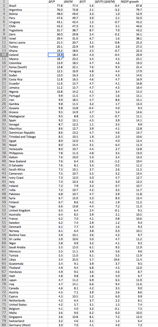
Now let’s return to the table in the previous post.  Notice that over 40 year periods the growth rates of M and P almost never differ by more than 10% (Libya’s the only exception.)  So one way of thinking about the correlations we see is to assume that there is some factor or factors causing the real demand for money to change, but their impact is rather modest, and doesn’t get bigger when the money growth rate gets really high.  So if real money demand is always changing by single digit annual rates over 40 year periods, then long run inflation will closely correlate with long run money supply growth, when the latter variable is growing really fast.  That’s why the QTM tends to do best in the high inflation cases, money demand changes pale by comparison.

Next let’s see if we can go a bit further, and explain the various discrepancies between money supply growth and inflation. We know that in an accounting sense it’s explained by changes in real money demand, i.e. real cash balances, but why would the public choose to hold more or less real cash balances?  What explains shifts in the real demand for money?

After Libya, two of the larger gaps are in East Asia, South Korea and Singapore.  In both cases money growth was much higher than inflation.  In an accounting sense that meant that the public in South Korea and Singapore were holding larger and larger cash balances.  Not just in nominal terms (as in Argentina) but even in real terms.  Their total holding of purchasing power rose by 9.3% per year in South Korea and 7.2% per year in Singapore, for many decades.  (The Singapore data is only for 1963-89.)  Why is that, why hold more purchasing power?  The answer is obvious—these economies grew very rapidly in real terms, and hence the real demand for money rose over time.  As the public became much richer and did much more shopping, they chose to hold larger real cash balances.

The sum of inflation and real GDP growth is NGDP growth.  If people hold larger real cash balances when real GDP grows, then perhaps the best way to think about the QTM is not to look at the correlation between money growth and inflation, but rather between money growth and NGDP growth.  In both Singapore and South Korea the money growth rate is much more closely correlated with NGDP growth than inflation. But if we insist on modeling inflation, then here’s what we have so far:

inflation = (Ms growth) – (real money demand growth)

Ms growth = f(Fed policy)

M/P growth = f(real GDP growth, other stuff)

Let’s try this conjecture.  When real GDP grows by X%, people choose to carry X% more real balances, to use for shopping, etc.  In that case, you’d expect the inflation rate to be equal to:

Inflation = Ms growth rate – real GDP growth rate + error term due to effects of other stuff

And that’s (almost) exactly what we found in the regression in the previous post.  Here I’ll first show a regression w/o real GDP growth, and then repeat the regression from the last post, with RGDP growth:

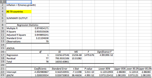
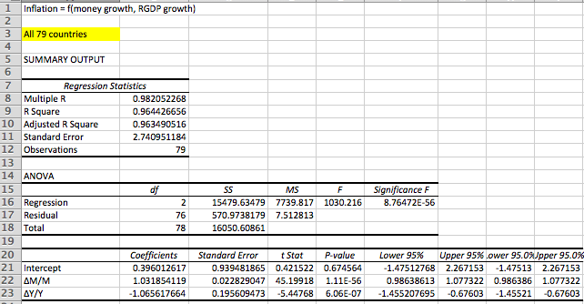
The coefficient on money growth is roughly one in both cases, and the coefficient on real GDP growth is roughly negative one in the second.  Growth is deflationary.  And the adjusted R2, which was already 95% in the simple regression of M and P, improves to over 96% when real GDP is added.

There is (or should be) nothing surprising about the finding that growth is deflationary, it’s the prediction of this very simple money demand model. It’s also the prediction of the AS/AD model—as the LRAS curve shifts to the right, the price level declines.  The only thing surprising is that so many people find this surprising.

By the way, suppose we label the “other stuff” with the letter V.  Then we have:

delta P = delta M – delta Y + delta V.

Look familiar?  It’s really just an identity; we need to explain the other stuff (V) to turn the Equation of Exchange into a model.

Let’s look for more hints in the data set.  Of the 79 cases, it seems like the vast majority show a money growth rate that is larger than the inflation rate.  That’s really not surprising, as almost every single country averaged positive RGDP growth over that period (except Guyana), and we’ve seen that positive economic growth holds down inflation, as the public desires to hold larger real cash balances.

Indeed the only surprise is that there were 12 cases where prices grew faster than the money supply, despite positive RGDP growth.  There were 12 cases where the inflationary impact of the “other stuff” was more than the deflationary impact of the real GDP growth.  We’ll model the other stuff in the next post, but first let’s briefly return to the issue of real GDP growth. Here are two questions:

1.  Can we assume that growth in M has no causal effect on Y in the long run?

2.  And if so, why are M and P positively correlated in the short run?

In the data set it looks like rapid money growth does not cause faster real GDP growth, at least in the long run.  The 10 highest inflation countries averaged 4.0% real GDP growth, and the 10 lowest inflation countries averaged 4.5% RGDP growth in the long run.  Money seems roughly long run superneutral, or perhaps hyperinflation is actually slightly negative for growth (as Mr. Ray Lopez has hypothesized.)

Then what’s going on in the short run?  Why does everyone think recessions reduce inflation and booms raise inflation? Here’s a hypothesis.  Suppose NGDP growth varies over time, due to monetary policy shocks.  And let’s assume that while money is long run superneutral, in the short run it has real effects–perhaps due to sticky wages and prices.  Thus in the short run, an increase in NGDP growth leads to both faster real GDP growth, and higher inflation.  In that case it would look like growth is inflationary, even though growth would actually be deflationary.  Thus if NGDP growth rose by 4%, and both RGDP growth and inflation rose by 2%, it would look like growth was inflationary.  But in fact the NGDP growth (i.e. monetary policy) was causing 4% higher inflation, ceteris paribus, and the extra 2% RGDP growth was holding down the inflation rate, limiting the increase in inflation to 2%.

If this is the way the world works then one might expect many cognitive illusions to form.  People would think growth was inflationary, whereas in fact it would be deflationary, as the regression in the previous post showed, and as our theoretical model predicts.  Procyclical inflation would reflect bad monetary policy (unstable NGDP growth) and inflation would be strongly countercyclical under a sound monetary policy regime (stable NGDP growth.)  If the central bank predicts that inflation will pick up during a boom period, they are predicting their own incompetence.

To summarize, it seems like the less restrictive version of the QTM is supported by the evidence.  If the money supply is increased by X%, this will lead in the long run to both prices and NGDP being X% higher than otherwise.  RGDP will be mostly unaffected.  But we’d still like to explain more of the discrepancies, the “other stuff.”  In the next post I’ll focus on those countries where inflation was higher than money growth, despite a growing real economy.  If you prefer to use the Equation of Exchange, then these are the rare cases where V rose by more than Y, over long periods of time.  We’ll also explain liquidity traps.

And in the post after that we’ll look at what happens when money supply growth rates are endogenous.  How does that affect the QTM?  It’s all there in the data set, if we look closely enough.  BTW, don’t think that this analysis has no implications for the low inflation world we live in today.  Monetary policy always and everywhere affects inflation and NGDP; we just need to figure out how to interpret what’s going on.

PS.  Some commenters pointed out that the data really should be first differences of logs.  That’s right, and I’m embarrassed to say that I don’t know if it is, or if it’s ordinary percentages (which is what I assumed when I had Patrick Horan calculate the NGDP growth rates.)  I’ll try to get an answer in a few days.

Update:  People asked for a graph.  Marcus Nunes has one for a very similar (but slightly different) data set.

I’m working on turning my blog into a book, and in order to do that I need to give readers an idea of how I ended up where I am today.  One obvious need is to explain how I adopted a quantity theoretic approach to monetary analysis, rather than some alternative like the interest rate approach.  For me it all goes back to the Great Inflation of the 1960s to the early 1980s.

As an aside, the quantity theory can be defined in several ways:

1.  An X% rise in M will be associated with an X% rise in P

2.  An X% rise in M will be associated with an X% rise in NGDP

3.  An X% rise in M will cause both P and NGDP to be X% higher than otherwise, in the long run.

The third definition is probably the most accurate, and the first is the least accurate.

The following data set (from a Macroeconomics textbook by Robert Barro) is so rich in information, that we will spend many posts investigating all the implications.  It shows average inflation, money growth and real GDP growth rates over 30 or 40-year periods around 1950-90, for 79 countries:

Right off the bat one notices the strong correlation between the growth rate of M (the monetary base) and P (the price level.) David Hume didn’t have this data set in 1752, but just using his brilliant mind he was able to figure out that if you double the money supply, the only long run effect is for prices to double.  Money is just a measuring stick.  For about 40 years Argentina and Brazil were doubling the money supply, on average, once every 14 months.  And prices were doubling just as Hume predicted.  All good, the Quantity Theory of Money (QTM) is triumphant.

Except it’s all downhill from here.  I’ve just provided the best possible data set for convincing you of the QTM.  Suppose I had only given you the bottom half of the data set?  Now the correlation is much harder to see.  Or suppose we’d looked at shorter time periods.  Again, not so good.  Or suppose we’d looked at countries at the zero bound?  Now the QTM would have major problems.

The key to understanding the QTM is to hold two thoughts in your mind at the same time.  In one sense the theory is logical, indeed blindingly obvious.  It’s incredibly powerful, incredibly true.  But in all sorts of situations it seems to fail.  That’s what we need to figure out.

Before moving on, let’s remind ourselves why it’s the bedrock of monetary theory, and why all other theories fall short.  In this data set we are doing the economic equivalent of when scientists expose objects to great heat, pressure, or speed, to get at the essential qualities.  We’re looking at what happens with very fast money growth

No other model can explain the correlations we see.  Yes, the growth in the money supply might have “root causes” elsewhere, such as budget deficits.  But you can’t figure out that Brazil and Argentina would have 75% inflation for 40 years, whereas Iceland would have 19% and the US would have 4% by looking at budget deficits, you need the money supply growth rates to even get in the right ballpark.  Note that some countries (the US in the 1970s) printed lots of money w/o big budget deficits.

Nor do interest rate models work.  Ironically the only interest rate model that would even come close is NeoFisherism, as the nominal interest rates in these countries would also be highly correlated with inflation.  But that model doesn’t tell you how you get those high nominal interest rates.  Again, you need money supply data.

Nor will an exchange rate model work.  Yes, the (depreciating) exchange rate for Brazil and Argentina was closely paralleling their inflation rate.  They saw the local currency price of US dollars rise at around 70% per year over those 40 years.  But that doesn’t explain how you cause the currency to depreciate so rapidly over 40 years. Again, you need money supply data. Both the Fisher effect and PPP are just appendages of the QTM.

Let’s finish today’s post with the first of several regressions that I’m going to give you–all provided by Patrick Horan of the Mercatus Center:

This is the Mona Lisa of macro regressions.  The t-statistic on money growth is 45.2. Yup, I’d say there’s some truth to the QTM.  The P-value?  One over . . . umm . . . how many atoms are there in the universe?  And the coefficient is pretty close to one, within two standard errors.  When you raise the money supply at 75%/year for 40 years, you’ll get roughly 75% inflation.

Later we’ll see there’s a reason the coefficient is slightly greater than one.  Can you guess? (It’s a very hard question.) But let’s finish up by noticing the coefficient on real GDP growth (delta Y).  You’ve all been taught that economic growth is inflationary.  The people at the Fed tell us that inflation will rise as we approach full employment.  Maybe it will, but not because growth is inflationary.  As you can see from the regression, economic growth is deflationary, indeed almost exactly as deflationary as money growth is inflationary.  So are the Keynesians wrong?

Yes they are!  And they are wrong in an interesting way.  Let’s suppose their predictions turn out right, and inflation does rise as we approached full employment.  Will I admit that I’m wrong?  Of course not!!  I’m an arrogant economic blogger.  Instead I’ll claim that this bizarre outcome is proof of the Fed’s incompetence.  They so botched monetary policy that they made inflation procyclical.  Indeed they do this so often that some of my commenters think this is natural.  Poor Mr. Ray Lopez found a dictionary somewhere that says inflation naturally falls during recessions and rises during booms.

And it’s all a myth.  Don’t worry, we’ll explain the mystery of deflationary growth in the next post.  And we’ll explain why the coefficient on money growth was a little bit bigger than one in the post after that.  All our money/macro questions are answered in this data set, if we know where to look.  Put on your David Hume thinking hat, you have lots more info to work with than he had. Indeed Milton Friedman became the second most famous economist of the 20th century mostly by figuring out how this data set allowed us to go “one derivative beyond Hume.”

PS.  Here are the two “money quotes” (pun intended) from Friedman:

Double-digit inflation and double-digit interest rates, not the elegance of theoretical reasoning or the overwhelming persuasiveness of serried masses of statistics massaged through modern computers, explain the rediscovery of money.” (1975, p. 176.)

As I see it, we have advanced beyond Hume in two respects only; first, we now have a more secure grasp of the quantitative magnitudes involved; second, we have gone one derivative beyond Hume.” Friedman (1975, p. 177.)

It seems that thousands of Mexicans . . . oops, I mean thousands of Vietnamese are pouring across the southern border to take the low wage jobs in factories that the Chinese are no longer willing to do.  Maybe China needs its own Donald Trump.

I’m not sure if the Mexicans will build our fence, but the Vietnamese are apparently building China’s newest Great Wall:

During a visit last year to the Chinese border town of Dongxing, small groups of Vietnamese workers could be seen building a 10-foot (3 metres) high border fence on the Chinese side. Ngoc Duc, 30, said he had come across the border illegally. He said he earned 100 yuan [$16] a day in China doing welding work on the fence, compared with about 200,000 dong ($9) a day in Vietnam.

“China is the best place to make money,” he said when asked if he feared being caught by Chinese authorities. “More and more of us will come.”

PS.  Ever get confused by all those Chinese provinces?  It’s much easier if you learn the 4 directions: bei (North), nan (south), dong (east) and xi (west.)  Also useful if you play Mahjong

Let’s start with Beijing, which means northern capital. Thus Nanjing means southern capital (before the communists took over.) Beijing is surrounded by Hebei province, which means north of the (Yellow) river.  Directly south is Henan, meaning south of the river, or literally “river south.”  Then Hubei, north of a big lake in central China. Then Hunan, lake south.  Then Guangxi and Guangdong, which means “expanse west” and “expanse east.”  Near Shanghai you see three provinces with “Jiang” which means long river, referring to the Yangtze.  Sichuan means 4 rivers, with “si” meaning 4.  Wait, do we now have three words for river?  Yes we do, but how many does English have?  Not sure about Yunnan, but Hainan means south sea.  And Shanghai means by the sea.

Going back up north we have Shanxi and Shandong, which mean west and east mountain.  Not to be confused with Shanxi is Shaanxi, right next door, which means west province, and my wife insists the pronunciation is totally different, although I can’t really hear it.

The Taiwanese use the old spelling system, so their capital city Taipei would be Taibei in Mandarin.  It’s on the north side of Taiwan.  On the south side is—you guessed it, Tainan.  And in the middle in Taichung, with chung meaning central.  What interesting names!! You can just describe where you are on the map in China, and 50% of the time you’ll accurately describe the place name in Chinese.  But chung is zhong on the mainland. Thus Zhongguo means “central country” (or middle kingdom if you prefer) and is the name of China.

Not quite sure why we call the Ivory Coast, “Cote d’Ivoire,” and Burma, “Myanmar”, but don’t call Germany, “Deutschland” or China, “Zhonggua”.