Archive for the Category Never Reason From a Price Change


Do low interest rates stimulate housing?

If you answer this question with a “yes”, then you are reasoning from a price change. I thought of this when reading the abstract to a paper by David W. Berger, Konstantin Milbradt, Fabrice Tourre, Joseph Vavra on monetary policy and mortgage interest:

How much ability does the Fed have to stimulate the economy by cutting interest rates? We argue that the presence of substantial household debt in fixed-rate prepayable mortgages means that this question cannot be answered by looking only at how far current rates are from zero. Using a household model of mortgage prepayment with endogenous mortgage pricing, wealth distributions and consumption matched to detailed loan-level evidence on the relationship between prepayment and rate incentives, we argue that the ability to stimulate the economy by cutting rates depends not just on the level of current interest rates but also on their previous path: 1) Holding current rates constant, monetary policy is less effective if previous rates were low. 2) Monetary policy “reloads” stimulative power slowly after raising rates. 3) The strength of monetary policy via the mortgage prepayment channel has been amplified by the 30-year secular decline in mortgage rates. All three conclusions imply that even if the Fed raises rates substantially before the next recession arrives, it will likely have less ammunition available for stimulus than in recent recessions.

People tend to refinance mortgages when long-term interest rates fall.  So what type of monetary policy generally causes long-term interest rates to decline?  I’d say the answer is contractionary, whereas the authors of this study seem to assume the answer is expansionary.  (I base this assumption on the first sentence of the abstract.  I have not read the entire paper, so it’s very possible I misinterpreted their claim.)

This is actually a complex question, and my reading of the evidence is that long-term rates will usually increase when monetary policy is made more expansionary (as in the 1960s and 1970s), but not always.  Of course it partly depends on how you define “expansionary”.

Consider the Fed announcements of January 2001 and September 2007.  In both cases, the Fed cut rates for the first time in years.  In both cases, the policy rate was cut by 0.5%, not the usual 0.25%.  In both cases, stocks soared on the unexpectedly expansionary policy news.  In both cases, long-term bond yields increased on the news (dramatically in January 2001), even as short term rates declined. If a highly liquid NGDP futures market had existed, then NGDP futures prices would have probably also increased.  On the other hand, you can also find lots of examples where short and long-term interest rates move in the same direction.  But the two cases I cited are important because they were so easily identifiable–the dramatic market responses at 2:15 pm seemed clearly linked to the Fed announcements.  “Identification” of policy shocks is easier in that case.

If I’m right that falling long-term bond yields generally reflect a contractionary monetary policy, then I think it’s a mistake to rely too much on the mortgage refinance channel when the Fed is trying to stimulate the economy.

I believe that monetary policy is always highly effective, even at zero interest rates.  We have lots of historical evidence to support that claim.  But if it is effective, it’s not because lower interest rates stimulate demand, rather it is because monetary stimulus increases the monetary base and/or reduces base demand, which boosts NGDP.  And higher NGDP leads to higher employment in a world with sticky wages.  In most cases, long term interest rates will also increase.

HT:  Tyler Cowen

Teaching money/macro in 90 minutes

A few weeks ago I gave a 90-minute talk to some high school and college students in a summer internship program at UC Irvine.  Most (but not all) had taken basic intro to economics.  I need to boil everything down to 90 minutes, including money, prices, business cycles, interest rates, the Great Recession, how the Fed screwed up in 2008, and why the Fed screwed up in 2008.  Not sure if that’s possible, but here’s the outline I prepared:

1.  The value of money (15 minutes)

2.  Money and prices  (20 minutes)

3.  Money and business cycles (25 minutes)

4.  Money and interest rates (15 minutes)

5.  Q&A (15 minutes)

Intro

Inflation is currently running at about 2%.  It’s averaged 2% since 1990.  That’s not a coincidence, the Fed targets inflation at 2%.  But it’s also not normal.  Inflation was much higher in the 1980s, and still higher in the 1970s.  In the 1800s, inflation averaged zero and there were years like 1921 and 1930-32 where it was more like negative 10%!

We need to figure out how the Fed has succeeded in targeting inflation at 2%, then why this was the wrong target, and finally how this mistake (as well as a couple freshman-level errors) led to the Great Recession.

1. Value of Money  

Like any other product, the real value of money changes over time.

But . . . the nominal price of money stays constant, a dollar always costs $1

Value of money = 1/P (where P is price level (CPI, etc.))

Thus if price level doubles, value of a dollar falls in half.

Analogy:

Year      Height    Unit of measure   Real height

1980      1 yard           1.0                1 yard

2018      6 feet            1/3               2 yards

Switching from yards to feet makes the average size of things look three times larger.  This is “size inflation”.  But this boy’s measured height increased 6-fold, which means he even grew (2 times) taller in real terms.

Year      Income    Price level  Value of money   Real Income

1980     $30,000        1.0               1.0               $30,000

2018    $180,000       3.0               1/3               $60,000

The dollar lost 2/3rds of its purchasing power between 1980 and 2018, as the average thing costs three times as much.  This is “price inflation”.  But some nominal values increase by more than three times, such as this person’s income, which means the income doubled in real terms, or in purchasing power.

Punch line:  Don’t try to explain inflation by picking out items that increased in price especially fast, say rents or gas prices, rather think of inflation as a change in the value of money.  Focus on what determines the value of money . . .

2.  Money and the Price Level

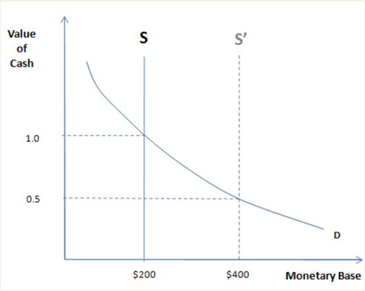
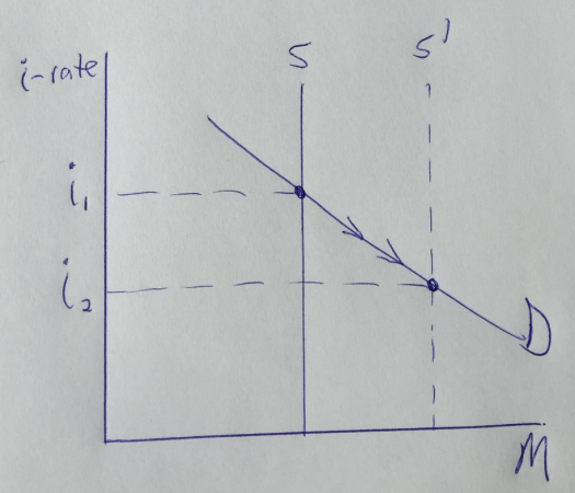
. . . which, in a competitive market is supply and demand:

Screen Shot 2018-08-02 at 7.11.51 PM

Demand for Money: How much cash people prefer to hold.

Who determines how much money you carry in your wallet?  You?  Are you sure?  Is that true for everyone?

Who determines the average cash holding of everyone in the economy?  The Fed.

How can we reconcile these two perceptions?  They are both correct, in a sense.

Helicopter drop example:  Double money supply from $200 to $400/capita

==> Excess cash balances

==>attempts to get rid of cash => spending rises => AD rises => P rises

==>eventually prices double.  Back in equilibrium.

Now it takes $400 to buy what $200 used to buy.  You determine real cash holdings (the purchasing power in your wallet), while the Fed determines average nominal cash holdings (number of dollars).

Punch line:  Fed can control the price level (value of money), by controlling the money supply.

What if money demand changes?  No problem, adjust money supply to offset the change.

Fed has used this power to keep inflation close to 2% since 1991.  Before they tried, inflation was all over the map.  After they tried, they succeeded in keeping the average rate close to 2%.  That success would have been impossible if Fed did not control price level.

But, inflation targeting is not optimal:

3.  Money and business cycles

Suppose I do a study and find that on average, 40 people go to the movies when prices are $8, and 120 people attend on average when prices are $12.  Is this consistent with the laws of supply and demand?  Yes, completely consistent. But many students have trouble seeing this.

Explanation:  When the demand for movies rises, theaters respond with higher prices.  The two data points lie along a single upward-sloping supply curve.

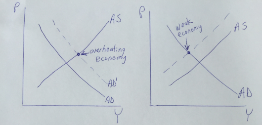
Implication:  Never reason from a price change.  A rise in prices doesn’t tell us what’s happening in a market.  It could be more demand or less supply.  The same is true of the overall price level.  Higher inflation might indicate an overheating economy (too much AD), or a negative supply shock:

Screen Shot 2018-08-02 at 7.26.42 PM

In mid-2008, the Fed saw inflation rise sharply and worried the economy was overheating.  It was reasoning from a price change. In fact, prices rose rapidly because aggregate supply was declining.  It should have focused on total spending, aka “aggregate demand”, for evidence of overheating:

M*V = P*Y = AD = NGDP

This represents total spending on goods and services.  Unstable NGDP causes business cycles.

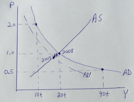
Example: mid-2008 to mid-2009, when NGDP fell 3%:Screen Shot 2018-08-02 at 7.43.04 PM

Here we assume that nominal GDP was $20 trillion in 2008, and then fell in 2009, causing a deep recession and high unemployment.

Musical chairs model:  NGDP is the total revenue available to businesses to pay wages and salaries.  Because wages are “sticky”, or slow to adjust, a fall in NGDP leads to fewer jobs, at least until wages can adjust.  This is a recession.

It’s like the game of musical chairs.  If you take away a couple chairs, then when the music stops several contestants will end up sitting on the floor.

The Fed needs to keep NGDP growing about 4%/year, by adjusting M to offset any changes in V (velocity of circulation).

Punch line:  Don’t focus in inflation, NGDP growth is the key to the business cycle

Why did the Fed mess up in 2008? Two episodes of reasoning from a price change:

1.  The 2008 supply shock inflation was wrongly viewed as an overheating economy.

2.  Low interest rates were wrongly viewed as easy money.

4.  Money and Interest Rates

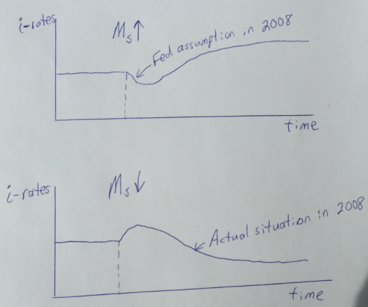
Below is the short and long run effects of an increase in the money supply, and then a decrease in the money supply.  Notice that easy money causes rates to initially fall, then rise much higher.  Vice versa for a tight money policy.

Screen Shot 2018-08-02 at 7.26.56 PMWhen the money supply increases, rates initially decline due to the liquidity effect. The opposite occurs when the money supply is reduced.

Screen Shot 2018-08-02 at 7.43.15 PMHowever, in the long run, interest rates go the opposite way due to the income and Fisher effects:

Income effect: Expansionary monetary policy leads to higher growth in the economy, more demand for credit, and higher interest rates.

Fisher effect:  Expansionary monetary policy leads to higher inflation, which causes lenders to demand higher interest rates.

In 2008, the Fed thought lower rates represented the liquidity effect from an easy money policy.

Actually, during 2008 we were seeing the income and Fisher effects from a previous tight money policy.

Don’t assume that short run means “right now” and long run means “later”.  What’s happening right now is usually the long run effect of monetary policies adopted earlier.

Punchline:  Don’t assume low rates are easy money and vice versa.  Focus on NGDP growth to determine stance of monetary policy.  That’s what matters.

(I actually ended up covering about 90% of what I intended to cover, skipping the yardstick metaphor.)

Erdogan reasons from a price change

[I wrote this a few weeks ago, and then decided not to post it.  After today’s news I changed my mind.]

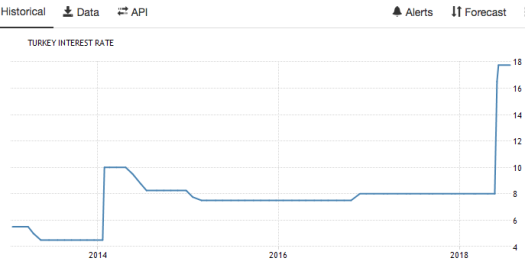
Turkish President Erdogan claims that the way to lower inflation is to have the central bank hold down interest rates.  How’s that theory working out?

Turkey’s central bank sharply lifted its annual inflation forecast on Tuesday to 13.4 per cent just a week after keeping interest rates on hold as it grapples with a weakening currency.

The move to raise the outlook from a previous forecast of 8.4 per cent in April comes amid concerns by investors about the independence of the central bank, which has come under pressure from Recep Tayyip Erdogan, the Turkish president, who is a self-declared “enemy” of high rates.

Murat Cetinkaya, the central bank governor, pushed back against claims that political interference is limiting his ability to tackle soaring inflation. Consumer price inflation hit 15.4 per cent in June — a figure three times higher the official 5 per cent target.

NeoFisherians correctly point out that a monetary policy that produces a sustained period of low inflation will be associated with low nominal interest rates.  But cutting the central bank policy rate does not cause inflation to fall, just the opposite.

As an analogy, ownership of a Ferrari is strongly correlated with being wealthy.  However purchasing a Ferrari does not cause one to be wealthier, just the opposite.

PS.  In fairness, the Turkish central bank did recently increase rates sharply.  But it was too late; years of holding rates at 8% let the inflation genie out of the bottle.  Now it’s playing catchup.

Screen Shot 2018-07-31 at 11.36.41 AM

Two examples of low interest rate monetary policies

I’ve done a number of posts comparing New Keynesian and NeoFisherian views on the relationship between monetary policy and interest rates.  Here I’d like to illustrate the problem with a picture, as people often have trouble understanding this issue.  It’s really hard to not reason from a price change.  It’s hard to stop thinking of interest rate movements as a “policy” rather than an outcome.

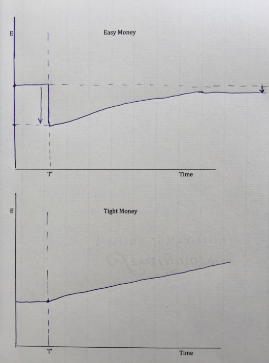
These two graphs show the path of the exchange rate (E) over time, under two different monetary policies.  In both cases a higher exchange rate (E rising) reflects domestic currency appreciation.  Importantly, both of these examples are “low interest rate policies”, when the central bank reduces interest rates to a lower level than before.  But case #1 is an easy money policy, whereas case #2 is a tight money policy:

Screen Shot 2018-05-26 at 4.51.28 PM

To focus on the essentials, I’d like to assume that a policy change occurs at time = T’, and that the following movement in the exchange rate is anticipated, once policy has shifted.  (The policy move itself was unanticipated beforehand.)

Notice that in both cases, the exchange rate is expected to appreciate after time = T’.  Because of the interest parity theory, this expected appreciation means that interest rates will be lower than before the policy change, when the exchange rate was stable and interest rates were the same as in the other country.  So from the interest parity theory we know that these two cases are both shifts to a lower interest rate policy.

But now let’s look at the long run impact of the two policies on the level of the exchange rate.  In case #1, the exchange rate ends up lower (depreciated) in the long run, despite the near-term expectation of appreciation.  Because of PPP, that means the policy is expected to increase the price level in the long run.  In other words, it’s an expansionary monetary policy.

In case #2, the exchange rate appreciates in the long run, yielding a lower price level.  That’s a contractionary policy.

Because the first case looks so convoluted—a currency that is expected to appreciate over time but still end up lower than before—you might think it represents the “weird and controversial model”.  Just the opposite, the first case is the New Keynesian model of easy money, and more specifically the Dornbusch overshooting version.  The second more straightforward case reflects the weird and controversial NeoFisherian model.  Just looking at the second graph, it’s easy to see how the NeoFisherians are able to get their result from mainstream mathematical models of the economy.

Here’s another way of thinking about the two cases.  In case #1, there is a one-time increase in the money supply (and/or reduction in money demand).  It reduces interest rates (due to the liquidity effect.)  But it also leads to expectations of a higher price level in the long run, due to currency depreciation and PPP.  Because prices are sticky in the short run, the effect of easy money is to initially depreciate the currency, not raise the price level in proportion.

In case #2, there is a permanent decrease in the growth rate of the money supply (and/or increase in money demand growth).  Because of the quantity theory of money, that leads to a permanent decrease in the inflation rate.  And because of the Fisher effect, the lower inflation leads to lower nominal interest rates.  And because of interest parity, lower nominal interest rates lead to an expected appreciation in the currency.  But you don’t even need the interest parity relationship.  By itself, the lower expected inflation combined with PPP leads to the expected appreciation in the currency.

So how does this help us to better understand the New Keynesian/NeoFisherian dispute?  It may be helpful to contrast the “highly visible” with the “highly important”.  The New Keynesians are focused on the highly visible, while the NeoFisherians are focused on the highly important.

The vast majority of specific, short-term decisions by central banks are better viewed as one-time shifts in the money supply, rather than permanent changes in the growth rate of the money supply.  Thus “easy money” announcements often make short-term interest rates fall, even as inflation expectations rise.  At the same time, the truly major moves in interest rates over time largely reflect longer-term changes in the growth rate of the money supply (and money demand—in more recent years).  Thus the low nominal rates in Japan are primarily due to tight money, not easy money.

Both the New Keynesian and the NeoFisherian models are wrong, as both sides engage in reasoning from a price change.  The correct (market monetarist) model says that low rates can reflect easy or tight money, and that one should not draw any inferences about the current stance of monetary policy by looking at interest rates.

If one cannot draw any inferences about the current stance of policy by looking at rates, can one draw any inferences at all?  I see two:

1.  On any given day, a decision by a central bank to cut rates by more than the market expected is usually (not always) expansionary.  It reflects “expansionary intent” and may be viewed as a signal by the central bank of a desire to make policy more expansionary.  This is, of course, consistent with New Keynesianism.  But it does not mean the current stance of policy is expansionary.

2.  When nominal interest rates fall persistently over a long period of time, it is usually (not always) evidence that monetary policy has been contractionary.  (This is more consistent with NeoFisherism).  But it does not mean that the current stance of monetary policy is contractionary.  As usual, Milton Friedman was decades ahead of the rest of the profession:

Low interest rates are generally a sign that money has been tight, as in Japan; high interest rates, that money has been easy.  .  .   .

After the U.S. experience during the Great Depression, and after inflation and rising interest rates in the 1970s and disinflation and falling interest rates in the 1980s, I thought the fallacy of identifying tight money with high interest rates and easy money with low interest rates was dead. Apparently, old fallacies never die.

In America, monetary policy in 2017 and 2018 became a bit more expansionary, despite higher rates.

Is an NGDP Phillips Curve somehow “wrong”?

I touched on this issue over at Econlog, but I’ll try again here in slightly a different way.

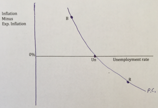
The original Phillips Curve from 1958 had nominal wage inflation on the vertical axis.  (Actually the original original PC was developed by Irving Fisher in the 1920s, and used price inflation.) Then American economists switched to price inflation in the 1960s.  In the 1970s and 1980s, economists accepted the Natural Rate Hypothesis and the expectations-augmented Phillips Curve was developed:

When inflation is higher than expected you are in a boom, and when it’s lower than expected you are in a recession.

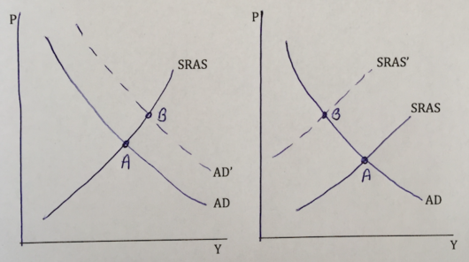
But inflation probably not the right variable, for standard “never reason from a price level change” reasons.  Higher inflation can reflect more AD, or less AS:

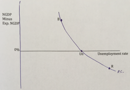
So what is the right variable?  As far as I can tell, the Phillips Curve should be using unexpected changes in NGDP:

So here’s my question to economics instructors.  Suppose you have an advanced topics chapter at the end of macro 101, which covers the standard Phillips Curve (using inflation), and discusses the Natural Rate Hypothesis and the importance of expectations.  Would it be acceptable to have a section at the very end of that chapter with the final two graphs shown here?  I.e., the two AS/AD graphs to show students the downside of using inflation as an indicator of whether the economy is overheating, and the NGDP version of the Phillips Curve to explain to students why more and more economists favor NGDP targeting.

Or is there something I am missing, which makes NGDP unsuitable for the vertical axis of a Phillips Curve?

PS.  The principles textbook I’m working on will be ready for consideration later this year, available for use in classes in the fall of 2019.