Is money too loose?  That might seem like a simple question, calling for a yes or no answer.  But it isn’t, because people wrongly think of monetary policy is a series of gestures, not a regime.

Our current regime has multiple goals, including an average inflation rate of 2%, and cyclical stability.  Often the two goals do not conflict, as in 2009.  But sometimes they do, like right now.

For example, monetary policy in Japan became more expansionary under Prime Minister Abe, producing slightly higher inflation and substantially higher NGDP growth.  I’ve argued that it’s still too contractionary because Japan remains well below its 2% inflation target.  Others say the labor market is now very strong (which is true) and that no further monetary stimulus is needed.  That’s also true, if you are focusing on the “stabilization” part of monetary policy.  But I believe Japan would still benefit from raising trend inflation high enough to escape the zero rate bound.

Recent Fed policy has given the US economy exactly the same sort of sugar rush as the Japanese felt after 2013.  Both NGDP growth and inflation are accelerating modestly.  From a “stabilization” perspective, policy may be too expansionary.  On the other hand, core PCE inflation is right at 2%, after a long period of underperformance.  From this perspective, policy is finally getting right on track.

Here’s another way of thinking about the dilemma.  The Fed’s dual mandate calls for above 2% inflation when unemployment is high, and below 2% inflation when unemployment is low.  The average rate should be 2%.  Unemployment is currently low, and hence the Fed should shoot for below 2% inflation.  But the Fed ran a tight monetary policy during the Great Recession and slow recovery, so if they run below 2% inflation right now they may lose credibility.  If you run below 2% inflation during both recessions and booms, then the average rate will obviously fall below 2%.

Right now, the Fed can either try to make its 2% long run inflation target credible at the expense of cyclical instability, or it can try to smooth out the business cycle at the expense of its long run 2% inflation target.  It cannot do both.

Or the Fed can adopt NGDPLT and do its best to run a countercyclical inflation rate.  Under NGDPLT, there are no “dilemmas”, just a clear target to shoot for, each and every day.

PS.  Demand-side fiscal policy is quite expansionary, but that doesn’t change anything I said here.  RGDP growth has been raised by supply-side reforms like the corporate tax cut, and that does interact with monetary policy by boosting NGDP growth (assuming the Fed targets inflation at 2%.)  In retrospect, Obama’s biggest policy mistake was not cutting the corporate income tax sharply in early 2009, instead of enacting the actual stimulus bill.  Of course if he’d had that ideology then he never would have gotten the Democratic Party nomination.

You’ve probably noticed that I no longer do as many posts on monetary policy.  That’s partly because I put my better posts over at Econlog and partly because there’s currently not much to talk about.  NGDP growth has been in the 3% to 5% range for 9 years, and I see no sign of anything changing in the near future (except perhaps a bit slower NGDP growth after this year, which is currently featuring above 4% growth.)  While boring is bad for me, it’s good for the economy.

Today, interest has turned to the question of when the next recession will occur.  The short answer is the same as always—no one can predict recessions.  But I’d like to talk about the issue anyway, since everyone seems interested in the question.

I’ve recently been catching up on David Beckworth’s podcasts, and listened to a very interesting discussion he had with Michael Darda.  Michael is a market monetarist who works in the investment area, and is known for having an excellent grasp of macroeconomics.  He knows the data quite well and he has a rare ability to interpret macro data correctly.  Lots of people are good at one, but he’s extremely good at both—no doubt partly due to his upbringing in Madison, Wisconsin.
At one point they began discussing the yield spread, which has been one of the better recession forecasting tools.  I’d like to put in my two cents worth.

As you can see from the following graph, the yield curve often inverts before a recession.  Here it’s important not to over interpret the correlation, as US expansions never last more than 10 years, and yield curves typically don’t invert until well into an expansion, and the lag between inversion and recession varies somewhat over time.  Furthermore, yield curves did not invert before recessions in the 1933-58 period.  Still it’s one of our most reliable forecasting tools.

Here are a few observations:

1.  Over at Econlog, I argued that while the yield spread is pretty good at predicting recessions, it’s much less good at indicating when money is too tight.

2.  It’s possible that the yield spread is reacting to changes in the unemployment rate.  Consider the following hypothesis.  The yield spread gets relatively flat whenever the unemployment rate falls to a level close to the natural rate of unemployment.  Let’s also assume that the unemployment rate falling close to the natural rate is a good predictor of recessions:

In that case we should be worried, as the unemployment rate has recently fallen to a level that is probably close to the natural rate.

Interestingly, there is one notable case when unemployment falling close to the natural rate did not lead to a recession.  In 1966, unemployment fell to 3.8% and there was no recession until 1970.  But that false signal is equally true of the yield spread, which also inverted in 1966.  Coincidence?

[On the other hand, the natural rate of unemployment is time varying (higher during 1975-95) and hard to measure, which makes the yield spread a better forecasting tool.]

When the unemployment rate is trending lower, it’s rational to expect the expansion to continue.  It may not always continue (consider 1981) but it’s a rational forecast.  And when unemployment is trending lower, the yield spread tends to be positive.  That’s because investors expect the future economy to be stronger than the current economy, and interest rates are highly correlated with the strength of the economy.

Conversely, when unemployment has fallen close to the natural rate, it’s no longer rational to expect lower unemployment in the future.  Indeed it’s quite likely that we’ll soon enter a recession.  That’s why the yield curve gets flat, and sometimes inverts.  In plain English, we never seem to achieve soft landings.  But Australia frequently does, and thus it’s not impossible.  The UK achieved a soft landing in 2001, and hence their 1990s expansion lasted until 2008.  If they can do it, so can we.

Memo to Jerome Powell:  Your mission, should you decide to accept it, is to avoid the hard landings that so often occur, but also avoid the 1966 scenario, where the Fed pulled up too soon, never landed at all, and instead soared off into the Great Inflation.  To do this, you need to avoid an excessively expansionary policy, which sometime triggers the inflation that later causes overly tight policy, and also avoid overly tight policy, which can directly cause a recession.  Let’s see . . . how about 4% expected NGDP growth?

Given that we’ve never had an expansion last for more that 10 years, you might wonder why I expect this one to go beyond a decade.  Well, until 2006-12 we’d never had a housing crash.  Until 2016, we’d never elected a lunatic as President.  Until 2018, we’d never adopted a wildly expansionary fiscal policy during a period of peace and prosperity.  None of those examples have any bearing on how long this expansion will last, rather they show that it’s really common for things to happen that have never happened before in the US.  And notice that other countries have had housing crashes before 2006, and lunatic presidents, and reckless fiscal policies during peace and prosperity.  That’s why I mentioned Australia and the UK (and there are many other such examples.) They provide an important clue that there is no inherent age limit on expansions.

Inductive reasoning can be useful, but must be handled with care.

PS.  The Hypermind NGDP prediction market is currently forecasting 4.8% NGDP growth from 2018:Q1 to 2019:Q1.  However, since the 2nd quarter is already in and growth was quite strong, this implies (annualized) 3.9% NGDP growth from 2018:Q2 to 2019:Q1.  Monetary policy is right on course.

PPS.  Because money is now boring, and my Trump posts are always stupid, please feel free to recommend other topics.  On the other hand, money is the only topic on which I have anything interesting to say.

A few weeks ago I gave a 90-minute talk to some high school and college students in a summer internship program at UC Irvine.  Most (but not all) had taken basic intro to economics.  I need to boil everything down to 90 minutes, including money, prices, business cycles, interest rates, the Great Recession, how the Fed screwed up in 2008, and why the Fed screwed up in 2008.  Not sure if that’s possible, but here’s the outline I prepared:

1.  The value of money (15 minutes)

2.  Money and prices  (20 minutes)

3.  Money and business cycles (25 minutes)

4.  Money and interest rates (15 minutes)

5.  Q&A (15 minutes)

Intro

Inflation is currently running at about 2%.  It’s averaged 2% since 1990.  That’s not a coincidence, the Fed targets inflation at 2%.  But it’s also not normal.  Inflation was much higher in the 1980s, and still higher in the 1970s.  In the 1800s, inflation averaged zero and there were years like 1921 and 1930-32 where it was more like negative 10%!

We need to figure out how the Fed has succeeded in targeting inflation at 2%, then why this was the wrong target, and finally how this mistake (as well as a couple freshman-level errors) led to the Great Recession.

1. Value of Money  

Like any other product, the real value of money changes over time.

But . . . the nominal price of money stays constant, a dollar always costs $1

Value of money = 1/P (where P is price level (CPI, etc.))

Thus if price level doubles, value of a dollar falls in half.

Analogy:

Year      Height    Unit of measure   Real height

1980      1 yard           1.0                1 yard

2018      6 feet            1/3               2 yards

Switching from yards to feet makes the average size of things look three times larger.  This is “size inflation”.  But this boy’s measured height increased 6-fold, which means he even grew (2 times) taller in real terms.

Year      Income    Price level  Value of money   Real Income

1980     $30,000        1.0               1.0               $30,000

2018    $180,000       3.0               1/3               $60,000

The dollar lost 2/3rds of its purchasing power between 1980 and 2018, as the average thing costs three times as much.  This is “price inflation”.  But some nominal values increase by more than three times, such as this person’s income, which means the income doubled in real terms, or in purchasing power.

Punch line:  Don’t try to explain inflation by picking out items that increased in price especially fast, say rents or gas prices, rather think of inflation as a change in the value of money.  Focus on what determines the value of money . . .

2.  Money and the Price Level

. . . which, in a competitive market is supply and demand:

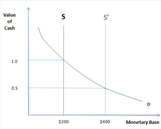
Demand for Money: How much cash people prefer to hold.

Who determines how much money you carry in your wallet?  You?  Are you sure?  Is that true for everyone?

Who determines the average cash holding of everyone in the economy?  The Fed.

How can we reconcile these two perceptions?  They are both correct, in a sense.

Helicopter drop example:  Double money supply from $200 to $400/capita

==> Excess cash balances

==>attempts to get rid of cash => spending rises => AD rises => P rises

==>eventually prices double.  Back in equilibrium.

Now it takes $400 to buy what $200 used to buy.  You determine real cash holdings (the purchasing power in your wallet), while the Fed determines average nominal cash holdings (number of dollars).

Punch line:  Fed can control the price level (value of money), by controlling the money supply.

What if money demand changes?  No problem, adjust money supply to offset the change.

Fed has used this power to keep inflation close to 2% since 1991.  Before they tried, inflation was all over the map.  After they tried, they succeeded in keeping the average rate close to 2%.  That success would have been impossible if Fed did not control price level.

But, inflation targeting is not optimal:

3.  Money and business cycles

Suppose I do a study and find that on average, 40 people go to the movies when prices are $8, and 120 people attend on average when prices are $12.  Is this consistent with the laws of supply and demand?  Yes, completely consistent. But many students have trouble seeing this.

Explanation:  When the demand for movies rises, theaters respond with higher prices.  The two data points lie along a single upward-sloping supply curve.

Implication:  Never reason from a price change.  A rise in prices doesn’t tell us what’s happening in a market.  It could be more demand or less supply.  The same is true of the overall price level.  Higher inflation might indicate an overheating economy (too much AD), or a negative supply shock:

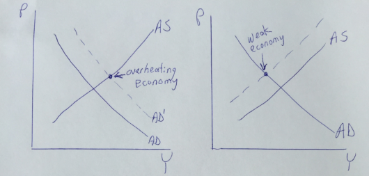
In mid-2008, the Fed saw inflation rise sharply and worried the economy was overheating.  It was reasoning from a price change. In fact, prices rose rapidly because aggregate supply was declining.  It should have focused on total spending, aka “aggregate demand”, for evidence of overheating:

M*V = P*Y = AD = NGDP

This represents total spending on goods and services.  Unstable NGDP causes business cycles.

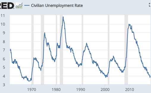
Example: mid-2008 to mid-2009, when NGDP fell 3%:

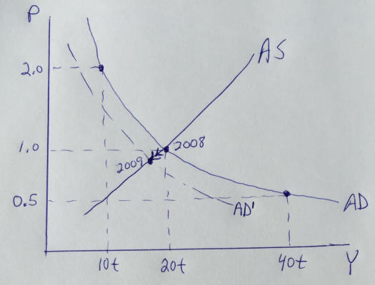
Here we assume that nominal GDP was $20 trillion in 2008, and then fell in 2009, causing a deep recession and high unemployment.

Musical chairs model:  NGDP is the total revenue available to businesses to pay wages and salaries.  Because wages are “sticky”, or slow to adjust, a fall in NGDP leads to fewer jobs, at least until wages can adjust.  This is a recession.

It’s like the game of musical chairs.  If you take away a couple chairs, then when the music stops several contestants will end up sitting on the floor.

The Fed needs to keep NGDP growing about 4%/year, by adjusting M to offset any changes in V (velocity of circulation).

Punch line:  Don’t focus in inflation, NGDP growth is the key to the business cycle

Why did the Fed mess up in 2008? Two episodes of reasoning from a price change:

1.  The 2008 supply shock inflation was wrongly viewed as an overheating economy.

2.  Low interest rates were wrongly viewed as easy money.

4.  Money and Interest Rates

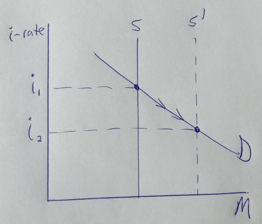
Below is the short and long run effects of an increase in the money supply, and then a decrease in the money supply.  Notice that easy money causes rates to initially fall, then rise much higher.  Vice versa for a tight money policy.

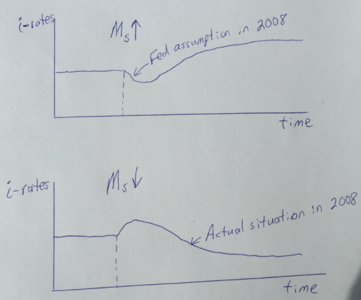
When the money supply increases, rates initially decline due to the liquidity effect. The opposite occurs when the money supply is reduced.

However, in the long run, interest rates go the opposite way due to the income and Fisher effects:

Income effect: Expansionary monetary policy leads to higher growth in the economy, more demand for credit, and higher interest rates.

Fisher effect:  Expansionary monetary policy leads to higher inflation, which causes lenders to demand higher interest rates.

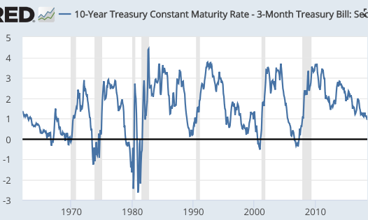
In 2008, the Fed thought lower rates represented the liquidity effect from an easy money policy.

Actually, during 2008 we were seeing the income and Fisher effects from a previous tight money policy.

Don’t assume that short run means “right now” and long run means “later”.  What’s happening right now is usually the long run effect of monetary policies adopted earlier.

Punchline:  Don’t assume low rates are easy money and vice versa.  Focus on NGDP growth to determine stance of monetary policy.  That’s what matters.

(I actually ended up covering about 90% of what I intended to cover, skipping the yardstick metaphor.)

[I wrote this a few weeks ago, and then decided not to post it.  After today’s news I changed my mind.]

Turkish President Erdogan claims that the way to lower inflation is to have the central bank hold down interest rates.  How’s that theory working out?

Turkey’s central bank sharply lifted its annual inflation forecast on Tuesday to 13.4 per cent just a week after keeping interest rates on hold as it grapples with a weakening currency.

The move to raise the outlook from a previous forecast of 8.4 per cent in April comes amid concerns by investors about the independence of the central bank, which has come under pressure from Recep Tayyip Erdogan, the Turkish president, who is a self-declared “enemy” of high rates.

Murat Cetinkaya, the central bank governor, pushed back against claims that political interference is limiting his ability to tackle soaring inflation. Consumer price inflation hit 15.4 per cent in June — a figure three times higher the official 5 per cent target.

NeoFisherians correctly point out that a monetary policy that produces a sustained period of low inflation will be associated with low nominal interest rates.  But cutting the central bank policy rate does not cause inflation to fall, just the opposite.

As an analogy, ownership of a Ferrari is strongly correlated with being wealthy.  However purchasing a Ferrari does not cause one to be wealthier, just the opposite.

PS.  In fairness, the Turkish central bank did recently increase rates sharply.  But it was too late; years of holding rates at 8% let the inflation genie out of the bottle.  Now it’s playing catchup.

David Beckworth has now done over 100 podcasts, but the recent interview with Kevin Erdmann would easily make the top ten in terms of general interest.  Kevin has a new book coming out soon (as well as a planned follow-up book), which put together many of the ideas in his blog posts on the real estate bubble and bust.  The podcast necessarily only covers a portion of this material, and I’ll just discuss a portion of the podcast.  But you should definitely get the book when it comes out, as it is loaded with lots of fascinating information that goes against the conventional wisdom.  And that’s because Kevin actually took the time to take a close look at the data.

One big theme is the “closed access” cities such as NYC, LA, the SF Bay Area and Boston.  These are the heart of the new, high-skilled information economy.  For the first time in history, however, we have been seeing people fleeing the engines of prosperity.  This is because of tight building restrictions that force out lower income workers as professionals move in, searching for jobs.  This worsens the economic prospects of low-income workers, and makes our overall economy less productive.

Another theme is that the housing bubble has been misinterpreted.  During the boom, it was higher income people who got the vast majority of mortgages in the closed access cities.  Large numbers of lower and moderate-income people were priced out and fled to the “contagion cities” such as Phoenix, Vegas, Riverside, Tampa and Miami, pushing up prices in those markets.  Contrary to what people assumed at the time, the high prices in closed access cities were not a bubble, rather a rational response to actual and expected rent inflation.  Consistent with Kevin’s view, prices in these cities have returned to bubble highs, despite the headwind of tighter lending standards than during 2006.  There were certainly not too many houses being built in those areas during the boom, rather NIMBYism caused too little construction.  And even in places like Phoenix it’s not clear the main problem was too many houses, as rent inflation kept rising even after the bubble burst.  At the national level, housing construction was not unusually high during the boom years, if you account for all types of housing.  Rather housing construction has been unusually low since 2007.

This is just the tip of the iceberg of Kevin’s work.  I believe Kevin’s story is basically correct, although I interpret the early housing bust (2006-07) slightly differently.  We both agree that tight money depressed housing prices during 2008-12, but Kevin thinks the Fed became a problem in 2006, partly due to somewhat tight money and partly due to Fed communication that the housing market had excesses that could lead to a substantial price drop.  I put a bit more weight on the post-2006 drop in expected future immigration.  The expected US population in 2050 is now 50 million lower than what the Census Bureau expected back in 2006, and 40 million of that decline had occurred by 2012.  The decline is mostly due to lower expected rates of immigration, although a falling birthrate also plays a role.  Recall that 2006 is the year that Bush’s immigration reform project failed and border controls were tightened.  Since then, net immigration from places like Mexico has fallen to a trickle, and it was this immigration that was helping to underpin the housing markets in the contagion cities.

I presume that immigration was not the only issue, but it might help to explain why housing began falling a bit earlier than NGDP growth.

PS.  Kevin’s book will be entitled: Locked Out: How the Shortage of Urban Housing is Wrecking our Economy