Archive for March 2017


Lars Christensen has a new website

One of the founding members of market monetarism (and the guy who provided the name) has a new website, called Markets and Money Advisory.

Each MM has their own special area of expertise, and I see Lars as the leading figure on the implications for MM for various European countries.  He had a career at a top Danish investment bank and is very knowledgeable about what’s going on across the Atlantic.

He’s also our most stylish presenter:

Screen Shot 2017-03-31 at 10.36.29 AMLars also informed me:

We are also launching a new – for pay – publication: Global Monetary Conditions Monitor (12 months for 2,000 euros).

Kocherlakota on Fed policy

Cloud Yip recently interviewed Narayana Kocherlakota:

Q: In the same paper, you have also suggested that in the reform of the Fed structure, we should strip New York Fed of its vote of FOMC. Can you walk us through your reasoning?

K: That’s more about the effectiveness of the monetary policy. The role of the non-New York Presidents is very clear in the process. They are the disruptive force of the groupthink that you would otherwise get in the Washington-based entity. We have just talked about there were only two dissents in the last 20 years out of the Board of Governors. That’s groupthink in work. The non-New York Presidents played a very valuable role on that dimension. Plus, they are very important in communicating with their own districts. So, I think non-New York regional Feds provided the two-way communication role and the independent thinking. They are very essential.

The New York Fed doesn’t play these roles. The New York Fed’s functions are mainly about gathering information among the financial markets and performing the Fed’s market functions. These are all important things. But their stuff works very closely with the Washington staff. There is really no way that the New York President can be independent of the Washington groupthink.

Also, though there are certainly some two-way communications that the New York President does, there is only a limited amount of that. But most of what New York is doing is on the information gathering in Wall Street and implementation of Fed’s policy in Wall Street.

On the flip side, given the closeness of the New York Fed and the Wall Street, having the New York Fed President votes in the FOMC really creates some misperceptions about Fed’s monetary policy. So, I just don’t think you get much benefit from having the New York Fed President votes. They are very close to the Wall Street, and they are actually located right in the Wall Street. It looks like Wall Street has a lot of say over monetary policy. I just don’t think the pluses outweighs the negatives.

Those are good points.  Peter Conti-Brown points out that one objection to Fed presidents voting is that this means important government policy is set by people who are not government employees.  This creates the impression that the Fed caters to the banking industry (and it’s probably not even constitutional).  One solution is to continue having Fed presidents vote, but make them government appointees picked by the President and confirmed by Congress.

This also caught my eye:

In a section of his book “The Courage to Act”, Ben Bernanke wrote about how three governors, Powell, Stein, and Duke, were the main influences behind initiations of the tapering in 2013. All that took place behind the scenes. The public has no idea of that was going on. I just don’t think that is a good way to make policies. Fed Independence does not mean opaqueness. The only way for the independence to survive is for the Fed to be transparent about how it makes the decisions that it is making.

Two of those hawks were Obama appointees.  This is why I think people obsess way too much about who Trump might appoint to the Fed.  It makes much less difference than you might imagine.  Imagine back in 2009 speculating who Obama might pick—would you expect it to be a couple of hawks who advocated tighter money in the midst of the weakest recovery in American history?

Mormons, Danes, and East Asians

I went to a public school in Madison, Wisconsin during the 1960s.  That’s one of America’s most egalitarian cities in one of the most egalitarian decades.  Only in retrospect do I realize what a “weird” place it was. If you had told me in 1969 that a white person’s prospects in life depended on how rich their parents were I would have had no idea what you were talking about.  To me, life seemed very simple.  We almost all went to the Madison Public Schools, and the few who didn’t mostly went to Catholic schools of roughly equal quality.  It seemed like success depended on some combination of being innately smart (or charismatic) and having a strong work ethic.  I did not even know anything about the socio-economic class of my fellow students—what difference would it make if their parents were janitors or doctors?  If college bound, we all tended to go to the UW, where tuition was $300/semester.  And those that could not afford that pittance could get student loans.  And college didn’t affect one’s income very much–a union job was just as good. I had two friends; the one from a low-income area was a better student than the one from a high-income area.  Other than those two, I knew nothing about the family background of students, which seemed completely irrelevant to life’s success.  (My uncle grew up in what we then called a “hillbilly family” in Kentucky, and was a distinguished professor at the University of Wisconsin.)

I’m not saying all this to try to convince you of anything.  Madison in the 1960s was a very unusual place, and I undoubtedly missed a lot that was important even back then.  But I tend to think of this background when reading the recent discussion of Raj Chetty’s work on income mobility.  Tyler Cowen links to Megan McArdle, discussing Chetty’s work on upward mobility:

There’s no getting around it: For a girl raised on the Upper West Side of Manhattan, Salt Lake City is a very weird place.

I went to Utah precisely because it’s weird. More specifically, because economic data suggest that modest Salt Lake City, population 192,672, does something that the rest of us seem to be struggling with: It helps people move upward from poverty. I went to Utah in search of the American Dream.

I’m pretty sure McArdle’s experience in high school was quite different from mine (it can’t have been any worse.)  Partly because New York was more diverse than Madison, and partly because (I assume) she’s more observant than I am, and far more than I was at age 14.  But Utah doesn’t seem weird to me.

Madison is not Mormon, and it does have a lot of heavy drinking, but otherwise both places are part of Nordic America, the North Central part of the US.  This map in Chetty’s paper shows higher levels of upward mobility (among whites) in lighter colors:

Screen Shot 2017-03-28 at 4.52.03 PM
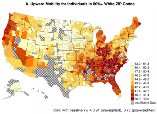
Actually, Madison’s on the fringe of Nordic America, the epicenter seems closer to South Dakota.  (I had one Scandinavian grandparent.)

At one point McArdle compares the upward mobility of Utah and Denmark:

The wide gulf between Utah and, say, North Carolina implies that we do, in fact, have a real problem on our hands. A child born in the bottom quintile of incomes in Charlotte has only a 4 percent chance of making it into the top quintile. A child in Salt Lake City, on the other hand, has more than a 10.8 percent chance — achingly close to the 11.7 percent found in Denmark and well on the way to the 20 percent chance you would expect in a perfectly just world.

Interestingly she doesn’t pursue that link any further.  Lars Christensen tipped me off to this fact:

Denmark supplied more immigrants to Utah in the nineteenth century than any other country except Great Britain. Most of these Danes–nearly 17,000–were converts to the LDS Church, heeding an urgent millennialistic call to gather to “Zion.”

Given that Denmark has less than 1% of Europe’s population, that’s a pretty interesting coincidence.  And other Scandinavian countries were also well represented:

Periodicals in their native language served combined audiences of Danes and Norwegians, and sometimes Swedes as well. The most successful of these was the Danish-Norwegian newspaper Bikuben (The Beehive), published in Salt Lake City from 1876 through 1935 (under LDS Church ownership in later years).

Whatever’s going on in North Central America, and Utah as well, I’m pretty sure it has something to do with Nordic culture.

The title of this post includes “East Asians”; what do they have to do with Utah?  The same Chetty paper has a table of mobility by metro area:

Screen Shot 2017-03-28 at 6.47.32 PM
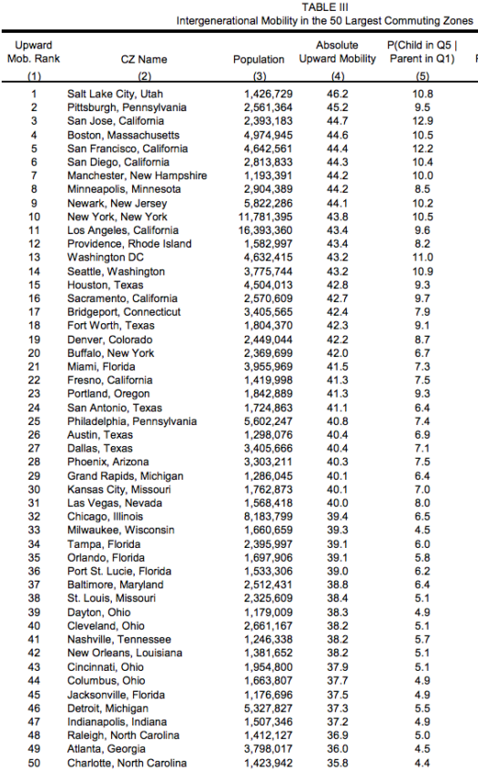
Notice that 3 of the top 6 cities are places in California with lots of upwardly mobile Asian families.

So let me finally get to the point.  I see a similarity between North Central America (including Utah) and East Asia.  In the not too distant past, both places were largely agricultural.  But in the 21st century global economy the big money is no longer in farmland, it’s in ideas.  Both areas have lots of upwardly mobile people who have successfully made the jump into the 21st century economy.  Like me!  (And my wife.)  Lots of other cultures, in America and elsewhere, seem to struggle with the demand of the 21st century.

In one sense, the success of East Asia is easier to explain, because they started from a far lower level.  When East Asia finally linked up with the global economy, they discovered that their cultures had a set of attributes that were well suited to achieving upward mobility—such as an emphasis on education, hard work, high saving rates, low crime rate, stable families, etc.  Many of these cultural attributes also show up in North Central America.  China is full of billionaires who started life as dirt-poor peasant farmers.  I’d guess that 90% of the world’s billionaires who grew up in abject poverty are Chinese, and roughly zero percent are American.

But why do white Americans from Iowa and Utah have more upward mobility than white Americans from other areas.  One possibility is that it’s easier to jump from the bottom 20% to the top 20% in places where those quintiles are not that far apart.

Lots of smart kids in the upward Midwest grew up in dead end small towns without much opportunity, but then used university education to make a jump to places where they could achieve much more success.

People on the two coasts tend to have a mental image of rural America as being “poor”.  But the upper Midwest contains lots of pretty big and successful family farms.  In the old days when America was more equal, talented people would have been much more content to stay in their region of the country.  If they moved, it more likely was in search of a better climate.  Why move from cold Wisconsin to cold Massachusetts when (during the 1960s) the incomes weren’t much different?  High tech barely existed back then.

PS.  What areas surprise you the most?  For me, it’s the low upward mobility of Michigan and western Oregon, and the fact that Louisiana has more mobility than the rest of the Deep South.

Ryan Murphy on state and local stimulus

Ryan Murphy has a new piece at Mercatus that discusses the problem of estimating spending multipliers using regional data:

Even if the central bank is perfectly competent and offsets the effects of fiscal stimulus entirely (meaning the multiplier at the national level is zero), these statistical methods when applied to subnational data still calculate the fiscal multiplier to be greater than one. Under conventional assumptions and settings where central banks credibly target certain nominal variables, any multiplier greater than zero should instead be interpreted as one region taking aggregate demand and jobs from another. In other words, a multiplier of greater than zero in one area implies a multiplier less than zero in another.

Unfortunately, most researchers seem to be aware of this problem:

Research employing these methods is published in elite academic journals such as American Economic Review and American Economic Journal: Economic Policy. Very rarely does it seriously address the negative externality problem. If it does, it often implies that states engaging in fiscal stimulus will provide a positive spillover for neighboring states. When the problem is referenced, it is noted as a small caveat deep within the paper. For instance, one paper states in its abstract that $100,000 of public outlays corresponds to 3.8 job years (implying a multiplier greater than one). This article has been cited 133 times as of September 2016, according to Google Scholar. Within the paper, however, the authors write, “given that the results from this cross-state approach do not incorporate equilibrium effects, cross-state multipliers, or the response of the monetary authority, we interpret this multiplier as only suggestive of the national multiplier of policy interest.” This interpretation entirely undercuts their point.

Now that we have a new administration determined to pursue tax reform and infrastructure spending, it’s worth reviewing where monetary offset does and does not apply.  Pundits often confuse the supply-side with the demand-side, when talking about the “growth” effects of “stimulus”.  If the stimulus is demand-side, then monetary offset probably prevents any meaningful effects.  But supply-side policies can still create growth, even with monetary offset.

Infrastructure spending is purely a demand-side policy as long as the infrastructure is still under construction.  Thus one should not expect any immediate impact on growth from spending more on big projects such as highways, bridges and airports. Once an infrastructure project is complete, it may (and I emphasize ‘may’) boost aggregate supply, and hence real GDP growth.  In my view, the supply-side effects of the sort of infrastructure package we are likely to see will be very small.  That doesn’t mean it’s not worth doing, just don’t expect a dramatic boost to GDP growth.

As of now, the GOP is still claiming that it intends to pursue revenue neutral corporate tax reform.  In that case, there would be no demand-side effects, so there would be nothing for monetary policy to offset.  If the tax reform boosts the supply side of the economy, it may also boost real GDP growth.  As with infrastructure, the long run effect may be greater than the immediate impact, as tax reform is likely to lead to more business investment.  In my view tax reform could have a stronger supply side effect than infrastructure spending, albeit still fairly modest in absolute terms.

PS.  I saw that the new Vegas football stadium was approved today.  When these stadium projects are sold to the voters, there are promises of multiplier effects from the spending of tax dollars.  Good luck.

According to Wikipedia, Vegas is just as sensitive to preserving its heritage as Boston:

The stadium as proposed is a domed stadium with a clear roof and silver and black exterior and large retractable curtain-like side windows facing the Las Vegas Strip. There is a large torch in one end that would house a flame in honor of the late Al Davis.[37] MANICA Architecture confirmed on March 28th, 2017 that a full nude strip club would be included into the stadium to honor the heritage of Las Vegas.

Does this project in some strange way remind you of a certain American politician?

Update:  I guess that Wikipedia quote has been corrected.  Shame on me for being so gullible.

Screen Shot 2017-03-28 at 5.40.39 PM

My vision of macro

The following Venn diagram helps to explain how I visualize macro:

Screen Shot 2017-03-26 at 3.17.11 PMThere are three basic fields within macro:

1.  Equilibrium nominal

2.  Equilibrium real

3.  Disequilibrium sticky wage/price (interaction)

I’ll take these one at a time.

1. Within equilibrium nominal there are important concepts:

A.  The quantity theory of money

B.  The Fisher effect

C.  Purchasing power parity

The first suggests that a change in M will cause a proportionate change in P.  The second suggests that a change in inflation will cause an equal change in nominal interest rates.  The third suggests that a change in the inflation differential between two countries will cause an equal change in the rate of appreciation of the nominal exchange rate.

All three concepts implicitly hold something constant; either the real demand for money, the real interest rate, or the real exchange rate.  In all three cases the concept is most useful when the money supply and price level are changing very rapidly, especially if those changes persist for long periods of time.

2.  Equilibrium real macro can be thought of as looking at economic shocks that do not rely on wage/price stickiness.  These include changes in population, technology, capital, preferences, government policies, weather conditions, taxes, etc.  These can cause changes in the real demand for money, the real interest rate, the real exchange rate, the unemployment rate, real GDP, and many other real variables.

3.  Disequilibrium macro looks at nominal shocks that cause changes in real variables, but only because of wage/price stickiness.  Thus because prices are sticky, an increase in the money supply will temporarily cause higher real money demand, a lower real interest rate, and a lower real exchange rate.  These changes occur even if there is no fundamental real shock hitting the economy.  The effects are temporary, and go away once wages and prices have adjusted.

If wages and prices are sticky then an increase in the money supply will also cause a temporary rise in employment and real output.

And that’s basically all of macro.  (This is how I’d try to explain macro to a really bright person, if I were given only 15 minutes.)

I also believe that understanding the implications of this three part schema makes one a better macroeconomist. Talented macroeconomists like Paul Krugman tend to have good instincts as to which real world issues belong in each category. Here’s my own view on a few examples. For simplicity, I’ll denote these three areas: nominal, real, and interaction:

1.  Most business cycles in ancient times were real, with some interaction.  The 1500 to 1650 inflation was nominal.

2.  Recessions such as 1893, 1908, 1921 and 1982 were mostly interaction.

3.  The Great Depression was all three.

4.  The Great Inflation was mostly nominal, especially in high inflation countries.

5. The 1974 recession was more “real” than usual.  Ditto for the WWII output boom.

6.  The real approach works best for short run shocks to specific industries such as housing and oil, plus long run growth.  The nominal approach works best for high inflation rates and long run inflation.  The interaction approach works best for real GDP fluctuations in large diversified economies.

7.  If one set of economists say the Japanese yen is too strong, and another set say it’s too weak, they are probably using different frameworks.  Those who say its too strong are using a nominal framework, and are likely worried about deflation.  A weaker yen would boost inflation.  Those who think the yen is too weak are using a real framework.  Rather than worry about deflation, they worry that Japan has a current account surplus.  These views seem to contradict, but it’s theoretically possible for both to be right.  Perhaps the nominal exchange rate for the yen is too strong, and the real exchange rate is too weak.  You would then weaken the nominal exchange rate by printing money, and strengthen the real exchange rate by reducing Japanese saving rates.  (I don’t favor the latter, just saying that’s the proper implication of the misguided worry about Japanese CA surpluses.)

8.  Don’t let your policy preferences drive your analysis.  Throughout all of my life, it’s been assumed that monetary shocks drive real output by causing changes in the unemployment rate.  Not changes in trend productivity growth or population growth or labor force participation or any number of other variables.  Money matters because it affects unemployment.  If the unemployment rate is telling you that monetary policy is no longer holding back growth, the proper response is not to double down on your belief that we need easier money and then look for new theories to justify it, but rather to conclude that whatever problems we still have are now “real”, not “interaction.”

A good macroeconomist knows that all three fields of macro are very important, and which models apply to each of the three fields, and which field is most applicable to each real world macro issue.