In this post I’m going to throw out a bunch of graphs, and ask for advice.  First let me briefly discuss real wage cyclicality.  Many of the early macroeconomists believed that real wages should be countercyclical.  They held a sticky-wage theory of the business cycle.  When prices fell sharply, nominal wages seemed to respond with a lag (even in 1921.)  Thus deflation temporarily raised real wages, even as unemployment was rising.

Real wages were quite countercyclical between the wars, but after WWII many studies found them to be acyclical, or even procyclical.  Most economists thought this was inconsistent with sticky wage models of the price level, and new Keynesian models ended up focusing on price stickiness and inflation targeting.  Greg Mankiw and Ricardo Reis have a 2003 paper that shows that you generally want to target the stickiest price.

In 1989 Steve Silver and I published a paper in the JPE that showed real wages were somewhat countercyclical during demand shocks and strongly procyclical during supply shocks. We suggested that this finding was supportive of sticky wage models of the cycle.  It even got cited in some intermediate macro texts (Mankiw’s textbook and also Bernanke’s.)  But after a while it was ignored.  In the graph below I show real wages during the post war years:

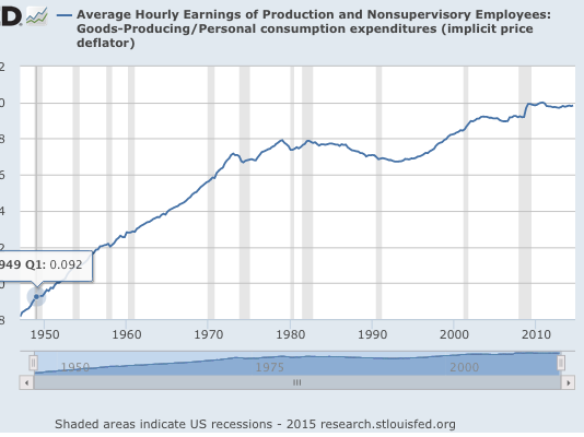
You can see why people didn’t find much cyclicality. And if you look closely you can also see some support for the paper I did with Steve Silver.  When real wages rise during recessions (1981-82, 2001, 2008-09) it’s a demand-side recession. When they clearly fall (1974, 1980) it’s a supply-side recession.  However there are some smaller demand-side recessions with almost no change in real wages.

Now let’s switch over to the “musical chairs” version of the sticky-wage model.  In the real wage model discussed above, firms lay off workers because production is less profitable at higher real wages.  In contrast, in the musical chair version of the sticky-wage model real wages don’t matter, what matters is revenue.  When firms receive less revenue they have less income to pay wages, so they employ fewer workers.  This would even apply to a socialist economy.  Imagine all firms were owned by workers, who shared revenues.  Also assume sticky nominal hourly wages.  Then when revenues fell, hours worked at the firms would decline. That might mean a shorter workweek (as occurred in 2008-09 in Germany) or it might mean fewer workers (as occurred in 2008-09 in the US.)

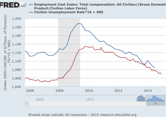
If we are looking to explain total hours worked, we might divide nominal wages by NGDP.  If trying to explain the unemployment rate, it makes more sense to divide nominal wages by NGDP/Labor force.  Previously I’ve showed that this cycle fits the musical chairs model quite well:

Unfortunately, we lack good wage data before 2006.  For earlier business cycles, all I could find was wages in goods-producing industries:

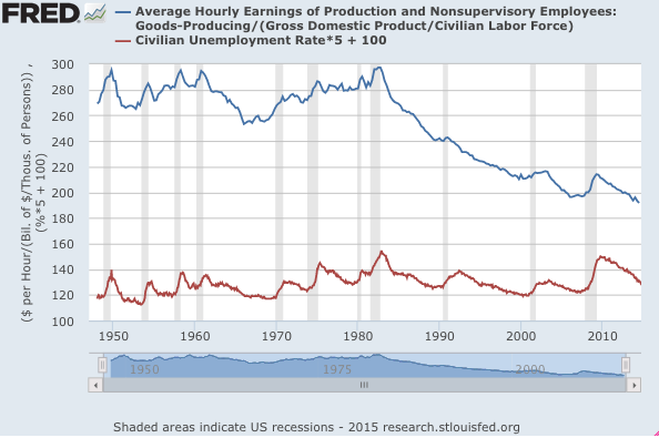
Notice that the ratio of hourly wages to NGDP/Labor force has a level trend from the late 1940s to 1982, and then plunges by a third.  That could reflect many factors, such as a change in hours worked per worker, but I think it more likely reflects three other factors:

1.  More fringe benefits (good for workers)

2.  Smaller share of NGDP going to workers (bad for workers)

3.  More inequality within labor income (bad for non-managerial factory workers)

But what really impressed me is the strong correlation between wages/(NGDP/LF) and the unemployment rate.  And by the way, even if you just used W/NGDP, you’d still see a strong correlation, as labor force changes are fairly “smooth.”  But there would be even more trend issues to deal with.  In my view, the weakest correlation appears to occur during the 1991 recession.  But even there you see a brief flattening of what had been a steep fall in W/(NGDP/LF) during the 1980s and 1990s.

Here’s one question.  How would you test for a correlation?  I suppose you could compute changes in W/(NGDP/LF) minus a ten year moving average of the same variable, and correlate that with change in unemployment.  Just eyeballing the graphs, I’d expect a reasonably close fit, even for 1990-91.

I know what you are thinking, how about the interwar years?  I could not find unemployment data, so I used industrial production.  Unfortunately that makes eyeballing the graph tougher as the predicted correlation is negative.  Also, the NGNP data for 1921 at the St. Louis Fred is total crap.  If someone over there is reading this, please replace your prewar NGDP estimates with Balke/Gordon, which is far superior, and goes back even further.

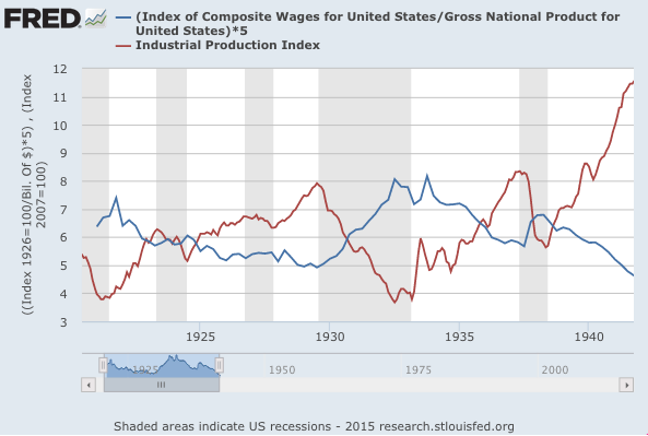
With the Balke/Gordon data, even 1920-21 would be a nice fit.  But you can see the W/NGDP ratio rise in 1929-33 and 1937-38 as IP falls sharply.

PS.  I was a bit surprised by the real wage series.  The fall in real wages from 1978 to 1993 didn’t surprise me—the rust belt took a toll on factory wages.  But the uptrend after 1993 was a bit better than I had expected, given all the gloomy articles on real wage growth.

You may wonder why I chose to name my chair at Mercatus the “Ralph Hawtrey Chair of Monetary Policy.”  Here are a few reasons:

1.  He was an early supporter of NGDP targeting, or something relatively close.

2.  He was an outstanding monetary economist.

3.  He was a moderate with pragmatic views.

4.  He had a sticky wage/monetary shock view of the cycle, and his views on the Great Depression were very close to mine (gold hoarding and artificial attempts to raise wages.)

5.  He believed in monetary offset of fiscal stimulus.

6.  He is well liked by people who disagree with each other on other issues, including David Glasner and George Selgin.  David dedicated his blog to Hawtrey.

Over at Econlog I have a much longer post with some quotes to back up these claims.

Let’s filter out the noise and look at three big turning points:

1.  The 1930s:  A deep and prolonged deflation from 1929 to 1933 was associated with sharply higher unemployment.  Economists drew the conclusion that policymakers needed to err on the side of expansionary policies, to prevent a repeat of the Great Depression.  They did.  And it worked.

2.  The Great Inflation (1966-81):  Higher and unstable inflation was associated with several problems such as unstable unemployment and distortions in capital markets.  Though not as bad as the Great Depression, economists agreed that the Fed needed to hold inflation at low and stable levels.  They continued to view business cycles as a significant problem, but noticed that the worst cycle in recent decades (the recession of 1981-82) was caused by a sharp slowdown in inflation. Thus inflation targeting should also stabilize growth, killing two birds with one stone.  They said we needed a Taylor-Rule type policy to stabilize inflation around 2%.  They succeeded.  No more Great Depressions and no more Great Inflations.

3.  The Great Recession:  Now economists noticed that even if inflation was pretty well anchored, we could have quite a bit of real instability.  Once low rates of inflation were achieved, it seemed like high and unstable unemployment was a much bigger problem than modest variations in inflation (say in the 0% to 4% range.)  Now we need a nominal aggregate that will stabilize output better than an inflation target, while still producing fairly well-anchored inflation over the business cycle.  That’s going to be NGDP targeting, or something closely related.   It will happen. And they will once again succeed.  And then no more Great Depressions and no more Great Inflations and no more Great Recessions.  That’s called progress.

Economists on both the left and the right are gradually moving to NGDPT.  Nick Rowe says that what convinced him is that it would have done much better in the recent severe business cycle. Severe problems are the problems you most want to prevent.  NGDPT does that.  Just today commenter W. Peden pointed to an endorsement of George Selgin’s (closely related) productivity norm by Allister Heath in The Telegraph.   He offers a conservative version of the idea, but center-left economists like Michael Woodford, Christy Romer and Jeffrey Frankel are also switching to NGDP targeting.

This isn’t rocket science–economists learn fairly predictable lessons from each major policy failure. This one is no different.  Central banks are conservative institutions so it will take a while for it to show up in the actual policy.  But you can be sure they are paying attention, and know that NGDPLT would have done better than IT in 2008-09. (Of course when I talk about central banks understanding what went wrong I am excluding the ECB.  There are in an entirely different category–still working on the lessons form the 1930s.)

The intellectual battle is almost over—time to consider what will go wrong under NGDPLT, and start working on the next improvement in monetary policy.  I vote for nominal aggregate labor compensation (per capita) targeting as the next iteration.

PS.  Check out Joe Leider’s blog, which makes some nice market monetarist arguments.

Here’s Paul Krugman’s latest:

David Beckworth has a good post pointing out that the Fed has been signaling all along that the big expansion in the monetary base is a temporary measure, to be withdrawn when the economy improves. And he argues that this vitiates the effectiveness of quantitative easing, citing many others with the same view. My only small peeve is that you might not realize from his list that I made this point sixteen years ago, which I think lets me claim dibs. Yes, I’m turning into one of those crotchety old economists who says in response to anything, “It’s trivial, it’s wrong, and I said it decades ago.”

Krugman may be 2 years older than me, but I’m more grouchy and reactionary. And thus I can’t help pointing to an article I did 21 years ago (5 years before Krugman’s admittedly far superior paper.)

[Note (1=r)n and (1+r)x are meant to be (1+r) raised to the power of n or x. I don’t know how to do superscripts.]

For example, suppose that at time=zero there is a nonpermanent currency injection that is expected to be retired at time=x. Then, if the real return from holding currency has an upper bound of r, the ratio of the current to the end-period price level (Px-n/Px) cannot exceed (1 + r)n. Furthermore, if real output is stable, it would not be expected that Px would be any different from Po. Both price levels would be determined by the supply and demand for money, as in the quantity theory. The existence of a maximum anticipated rate of deflation (r) has the effect of placing a limit on the size of the initial increase in the price level. No matter how large the original currency injection, the price level at the time of the currency injection cannot increase by more than a factor of (1+r)x. Furthermore, these restrictions on the time path of prices can be established solely on the basis of the future time path of the quantity of money, without any reference to fiscal policy. It is this quantity-theory model that is applicable to the colonial episodes of massive and nonpermanent currency injections. . . .The impact of U.S. monetary policy during the period from 1938 to 1945 provides a good illustration of the preceding hypothesis. Between 1938 and 1945 the currency stock increased by 368 percent while prices (the GNP deflator) increased by only 37 percent. There was no depreciation in the dollar (in terms of gold.) Although real output grew substantially, the ratio of currency to nominal GNP increased from .062 to .132. Why was the public willing to hold such large real balances?

Although the U.S. did not experience deflation following World War II (as it had following previous wars), surveys indicate that deflation was anticipated. During the entire period from 1938 to 1946, the three-month Treasury Bill yield never rose above 1/2 percent. The fact that massive currency injections (associated with expectations of future deflation) were able to drive the nominal interest rate down close to zero, is at least consistent with the modern quantity-theory model I have described.

And stay off of my lawn!

Update:  David Glasner found an even older example.  (I’m sure there are dozens out there.) But I’d quibble slightly with this:

For one thing, reasoning in terms of price levels immediately puts you in the framework of the Fisher equation, while thinking in terms of current and future money supplies puts you in the framework of the quantity theory, which I always prefer to avoid.

I can’t help pointing out that the Quantity Theory, the Fisher effect, and PPP are three very similar theories, which share almost exactly the same strengths and weaknesses.  And let me add that all three have enormous strengths and massive weaknesses.  (Yes, the Fisher effect isn’t actually a theory, but you can imagine an associated theory that says nominal interest rates change one for one with inflation.  Or if you prefer you can compare the Fisher equation with the very similar MV=PY equation.)

These three theories say the real interest rate, the real demand for money, and the real exchange rate are stable.  All three theories are far more useful at double-digit inflation rates than single-digit inflation rates.

A commenter sent me the following:

This slim volume describes a weighty and wonderful event. In 1920, the American economy entered what would presently be diagnosed as a depression. The successive administrations of Woodrow Wilson and Warren G. Harding met the downturn by seeming to ignore it””or by implementing policies that an average 21st century economist would judge disastrous. Confronted with plunging prices, incomes and employment, the government balanced the budget and, through the newly instituted Federal Reserve, raised interest rates. By the lights of Keynesian and monetarist doctrine alike, no more primitive or counterproductive policies could be imagined. Yet by late 1921, a powerful, job-filled recovery was under way. This is the story of America’s last governmentally unmedicated depression.

Sometimes it seems like everyone wants to pick on the monetarists, including to some extent even market monetarists.  Monetarism is ridiculed by Keynesians, Austrians, MMTers, Real Business Cycle supporters, fiscal theory of the price level proponents, etc., etc. It seems out of date, with not many young supporters.  It allegedly “failed” in the 1979-82 monetarist experiment, even though:

1.  That period successfully broke the back of inflation, as the monetarists predicted and others doubted, especially given the Reagan fiscal stimulus.  It led to a severe recession, as the monetarists predicted.  And it was followed by a strong recovery, as the monetarist predicted (but the Keynesians thought unlikely without a rise in inflation.)

2.  Furthermore, the policy of 1979-82 was not truly monetarist (money growth varied), and the monetarists would never have expected velocity to be stable during a period of rapid disinflation. Their argument was that V would stabilize in the long run, if money growth were stable in the long run.  That was never tried.

I find even that weaker claim to be dubious, which is one reason that I am not a traditional monetarist. And of course Friedman made some bad predictions in the 1980s (but since when do bad predictions discredit a model?) Nonetheless, let’s give monetarists their due; contrary to the implication of the quotation above, Friedman and Schwartz’s Monetary History does explain the depression of 1921:

M2 money supply:

May 1920 peak:  $30,304 million.

Sept. 1921 trough:  $27,830 million

December 1922:  $31,920 million

Monetarists would predict a steep recession and fast recovery.  And that’s what happened.

PS:  Rereading the quote, it doesn’t actually say the monetarists failed to predict a fast recovery, but I sort of think that was implied.  Did I misinterpret the quotation? How would the average person interpret the quote?

PPS.  I have not read Grant’s book, but I do believe the 1921 depression is a good example of the natural recuperative powers of a free market economy.  In that sense, it could be viewed as being inconsistent with old Keynesianism, as well as modern variants that say wage cuts will make the depression worse, and that massive fiscal stimulus is needed.  Of course Keynesianism is a slippery critter, which is hard to pin down.  They would probably point to the lack of a zero bound problem. They mention positive interest rates when convenient (1921) but ignore positive interest rates when inconvenient (eurozone 2008-12.)