In several recent posts Tyler Cowen has tried to draw a distinction between how much wealth we believed we had, and how much wealth we really had.  I was somewhat skeptical of his argument, but also thought it had some merit.  Indeed in an earlier post (not posted yet!) I tried to distinguish between wealth we correctly thought we had, which was later lost due to bad policy (1929), and wealth we thought we had, that we never really had (2006.)  Now I have doubts about my argument, indeed I think we might both be wrong.  But I’m not sure.

Consider the following 5 scenarios:

1.  The bank makes a typo, which leads you to believe you have more money than you actually have.  The typo is eventually corrected.

2.  Your family believes it owns 10 1933 $20 gold pieces, worth $80 million.  Later you find out the government has a different view.

3.  The public believes it has lots of housing wealth in 2006, but there was never any prospect that these values could be maintained.

4.  The public believes it has lots of housing wealth in 2006, but later an immigration crackdown followed by tight money reduces housing prices.

5.  The public believes it is very wealthy in 1929, but later the Fed cuts NGDP in half and caused mass unemployment.

A few days ago I thought there was a clear distinction between case 1 and case 5.  Now I don’t know where to draw the line.  Indeed I don’t know if there is a line to be drawn.

I’d like to say the public really was wealthy in 1929, and that later decisions by the Fed destroyed that wealth.  But is that a scientific way of looking at things?  At levels about subatomic particles, we tend to assume that things follow deterministic laws.  Why couldn’t someone argue:  “That national wealth in 1929 was never real, because the Fed is a part of our economy.  It was a dysfunctional institution in 1929, so it was only a matter of time before they screwed up.  We just didn’t know it yet.”

Rorty argued that when people say “Most people think X is true, but I believe Y is true,” they actually mean “most people think X is true, but I predict that in the future people will come to believe Y is true.”  Rorty saw no distinction between what is true, and what we believe is true.

Rorty also believed; “That which has no practical implications, has no philosophical implications.”  So what are the practical implications of the distinction between believing one is wealthy, and actually being wealthy?  Obviously society acts on the basis of beliefs.  So for most people it is a distinction without any significance.  Like the difference between saying I believe X, and I believe X is true.   On the other hand the skeptic who believes the wealth is phony (i.e. predicts it will later be seen as phony), would obviously see practical implications for his belief.  Indeed policy implications.

Imagine I’m debating Tyler Cowen on the question of whether the 2006 wealth was real in 2006.  What’s at stake?  I might argue that the wealth was 100% real, but later policies like immigration crackdown and tight money reduced the wealth later on.  The practical implication is that we might want to reconsider those policies.  Or, one could argue that the extra wealth was only 40% real and the other 60% was irrational exuberance.  In that case the policy implication might shift slightly.  It doesn’t mean easier money couldn’t have helped a bit, but you’d also want to put in place banking regulations robust enough to prevent housing bubbles from damaging the banking system.  Indeed you might also want to do that if the problem was 100% the Fed’s fault, but the necessity would be greater if optimal monetary policy couldn’t solve the problem.

Are we rich if we believe we are rich?  I can’t answer that question.  Rorty would say beliefs are all we have.  Yet he also allows for dissenting voices.  Just because most people get swept up in the housing bubble, and believe ranch houses in San Bernardino are worth $500,000, doesn’t mean Shiller, Krugman, Baker and Roubini have to believe that.  One the other hand, current market values have a very practical implication, they’re what we can sell things for.  In that sense they are real.

Each day that goes by we find out that the previous day’s value of the S&P 500 was wrong, as new information comes in.  Or maybe it was right; maybe it was “true,” based on what we knew at the time.  What’s the TRUE value of the S&P 500?  God only knows.

PS.  I just noticed an interesting shift in wording between the first and second posts that I linked to above.  First post:

We were not as wealthy as we thought we were.

And second post:

We are not as wealthy as we thought we were

See the difference?  If applied to someone in 1933 talking about 1929, I’d have once said the first was false, and the second was true.  Now I don’t know what to think.  I wish Rorty was still alive to help me out.  Now I feel alone in the universe, with no one to provide true answers.

PS.  The second Cowen post that I linked to above didn’t make sense to me.  I left a comment over there—maybe someone can explain the connection to AD.

Sometimes I become convinced that Paul Krugman made a mistake, and then when I go back and reread his post I find that he used his words very carefully, to artfully avoid being wrong while creating a misleading impression.  I was thinking about all his posts that claimed fiscal stimulus didn’t fail, because it wasn’t tried.  I recall that he kept pointing to graphs showing that declines in S&L government output roughly offset increases in federal output.  But what about taxes and transfers?  Aren’t they also fiscal stimulus?  When I went back and looked at one of the posts, here’s the conclusion I read:

But if they won’t say it, I will: if job-creating government spending has failed to bring down unemployment in the Obama era, it’s not because it doesn’t work; it’s because it wasn’t tried.

OK, I guess I can buy this.  After all, back in 2008 and 2009 Krugman had some posts pointing out that tax cuts were much less effective stimulants than government consumption and investment, at least according to some Keynesian models.  I don’t entirely agree with those models, but it’s a defensible argument.

But here’s my problem.  If taxes and transfers don’t count for much in 2009, then shouldn’t they also be disregarded in 1937?  I’m referring to the famous Keynesian explanation for the 1937-38 depression, one of the most severe in US history.  Keynesians often point to the tightening of fiscal policy that occurred in 1937 as the key factor that aborted the recovery.  But here’s the problem with that explanation.  Fiscal policy wasn’t all that contractionary in absolute terms, and more importantly the big changes in fiscal stimulus occurred in the area of taxes and transfers–the exact area that Krugman thinks are relatively unimportant.

The reduction in the budget deficit mostly reflected two factors.  First, the large one-time “bonus” payments made to WWI vets in 1936 (an election year) was not repeated in 1937.  And a 2% payroll tax was instituted to pay for Social Security in January 1937.  As far as I know those are the major contractionary moves.  But it was always understood that the 1936 bonus payments were a one-time deal.  How could that have caused a severe stock and commodity crash in late 1937, as well as a sharp plunge in industrial production in late 1937?

I found the following data from Thayer Watkins at SJSU:

Year   RGDP   Cons.  Inv.   Gov.   Exp.  Imp.  Balance

1934  641.1  519.0  31.5  127.3  21.4  31.1  -9.7

1935  698.4  550.9  58.0  131.3  22.6  40.7  -18.1

1936  790.0  606.9  75.5  152.5  23.7  40.2  -16.5

1937  831.5  629.7  94.0  147.0  29.9  45.3  -15.4

1938  801.2  619.5  61.3  157.8  29.6  35.2  -5.6

I just don’t see it.  Government output does decline slightly in 1937, but is still far higher than 1934 and 1935.  If you apply a multiplier of 1.6, it should have reduced GDP by about 1%.  But RGDP rose more than 5% in 1937.  Then in 1938 government output rises by twice as much as it fell in 1937, and RGDP plunges by almost 4%.  (BTW, we should be using NGDP figures, but everyone else uses RGDP, and the qualitative results would be similar either way.)

The 1938 depression had two causes, or perhaps one proximate cause and two deeper causes.  The proximate cause was a sharp increase in real labor costs.  Nominal labor costs rose sharply in 1937, due to a powerful union drive after the Wagner act, which rapidly doubled union membership and led to a wave of major strikes.  The payroll tax also slightly boosted nominal labor costs (I believe by 1%, but am not certain.)  Because wholesale prices were pretty high in the spring and summer of 1937, at first the wage boost merely led to a sharp slowdown in growth.  But then prices plunged due to a worldwide bout of gold hoarding, which increased the purchasing power of gold.  This tightened US monetary policy and caused the WPI to fall about 9% between mid-1937 and mid-1938.  Now two factors were driving up real wages, higher nominal wages and lower prices.  A supply shock and a demand shock.  Output plunged.  Severe slumps almost always have multiple causes.

So which is it?  Is Krugman wrong about 2009?  Or is he wrong about 1937?  Keynesians can’t have it both ways.

BTW, I eventually did find the quotation I was looking for, in another Krugman post:

The Obama fiscal stimulus more or less evaporates when you look at it closely, and take state and local cutbacks into account; basically, all it did was to keep overall fiscal policy from being outright contractionary.  (italics added)

I feel like that poor hunter trying to nab the roadrunner.  He usually gets away, but once and a while I catch him.

Update:  Many commenters argued that Krugman cited both a contractionary fiscal policy, and a contractionary monetary policy.  True, but irrelevant.  I’m saying that if fiscal policy was contractionary in 1937-38, then you really need to include taxes and transfers.  But in that case it was expansionary in 2009-10.

Paul Krugman and I both use a similar framework to analyze monetary policy.  Temporary monetary injections don’t have much effect; stimulus comes from injections that are expected to be permanent.  I thought it might be interesting to review just how similar our views are, given the small but important differences in how we interpret this framework.

This is from Krugman’s justifiably famous 1998 paper “It’s Baaack“:

One often hears, for example, that the real problem is that Japan’s banks are troubled, and hence that the Bank of Japan cannot increase monetary aggregates; but outside money is still supposed to raise prices, regardless of the details of the transmission mechanism. In addition to the problem of bad loans, one often hears that corporations have too much debt, that the service sector is overregulated and inefficient, and so on. All of this may be true, and may depress the economy for any given monetary base – but it does not explain why increases in the monetary base should fail to raise prices and/or output. One way to say this is to remember that the neutrality of money is not a conditional proposition; money isn’t neutral “if your banks are in good financial shape” or “if your service sector is competitive” or “if corporations haven’t taken on too much debt”. Money (which is to say outside money) is supposed to be just plain neutral.

So how is a liquidity trap possible? The answer lies in a little-noticed escape clause in the standard argument for monetary neutrality: an increase in the money supply in the current and all future periods will raise prices in the same proportion. There is no corresponding argument that says that a rise in the money supply that is not expected to be sustained will raise prices equiproportionally – or indeed at all.

.  .  .

Suppose that we start with a [flexible price] economy . . .  and then imagine an initial open-market operation that increases the first-period money supply.  (Throughout we imagine that the money supply from period 2 onwards remains unchanged – or equivalently that the central bank will do whatever is necessary to keep the post-2 price level stable). Initially, as we have already seen, this operation will increase the price level and reduce the interest rate. . . . But what happens if the money supply is increased still further – so that the intersection of MM and CC is at a point like 3, with a negative nominal interest rate?

The answer is clearly that the interest rate cannot go negative, because then money would dominate bonds as an asset. What must therefore happen is that any increase in the money supply beyond the level that would push the interest rate to zero is simply substituted for zero-interest bonds in individual portfolios (with the bonds being purchased by the central bank in its openmarket operation!), with no further effect on either the price level or the interest rate. . . .

A good way to think about what happens when money becomes irrelevant here is to bear in mind that we are holding the long-run money supply fixed at M*, and therefore also the long-run price level at P*. So when the central bank increases the current money supply, it is lowering the expected rate of money growth M*/M, and also – if it does succeed in raising the price level – the expected rate of inflation P*/P. Now what we know is that in this full employment model the economy will have the same real interest rate whatever the central bank does. Since the nominal interest rate cannot become negative, however, the economy has a minimum rate of inflation or maximum rate of deflation.

Now suppose that the central bank in effect tries to impose a rate of deflation that exceeds this minimum – which it does by making the current money supply M large relative to the future supply M*. What will happen is that the economy will simply cease to be cash-constrained, and any excess money will have no effect: the rate of deflation will be the maximum consistent with a zero nominal rate, and no more.

Great stuff.  In a 1993 paper on colonial American currency, I developed a similar idea.  Here’s a few passages from that paper:

[note (1=r)n and (1+r)x are meant to be (1+r) raised to the power of n or x.]

For example, suppose that at time=zero there is a nonpermanent currency injection that is expected to be retired at time=x.  Then, if the real return from holding currency has an upper bound of r, the ratio of the current to the end-period price level (Px-n/Px) cannot exceed (1 + r)n.  Furthermore, if real output is stable, it would not be expected that Px would be any different from Po.  Both price levels would be determined by the supply and demand for money as in the quantity theory.  The existence of a maximum anticipated rate of deflation (r) has the effect of placing a limit on the size of the initial increase in the price level.  No matter how large the original currency injection, the price level at the time of the currency injection cannot increase by more than a factor of (1+r)x.  Furthermore, these restrictions on the time path of prices can be established solely on the basis of the future time path of the quantity of money, without any reference to fiscal policy.  It is this quantity-theory model that is applicable to the colonial episodes of massive and nonpermanent currency injections. . . .

The impact of U.S. monetary policy during the period from 1938 to 1945 provides a good illustration of the preceding hypothesis.  Between 1938 and 1945 the currency stock increased by 368 percent while prices (the GNP deflator) increased by only 37 percent.  There was no depreciation in the dollar (in terms of gold.)  Although real output grew substantially, the ratio of currency to nominal GNP increased from .062 to .132.  Why was the public willing to hold such large real balances?

Although the U.S. did not experience deflation following World War II (as it had following previous wars), surveys indicate that deflation was anticipated.  During the entire period from 1938 to 1946, the three-month Treasury Bill yield never rose above 1/2 percent.  The fact that massive currency injections (associated with expectations of future deflation) were able to drive the nominal interest rate down close to zero, is at least consistent with the modern quantity-theory model I have described.

In both our papers the equilibrium real interest rate sets the maximum rate of expected deflation.  Krugman recognized that the equilibrium real interest rate might be negative (and thus we might have a liquidity trap at positive expected rates of inflation.)  Oh, and although my paper came first, his is 100 times better.

In future posts I’ll discuss why we interpret this framework differently.  But at least we agree that the quantity of money drives the price level in the long run.

And just so you won’t think there’s anything new under the sun, here’s some Congressional testimony from 1932 involving New York Fed President Harrison and Representative Goldsborough (proposing a price level targeting bill.)  Notice how it weirdly echoes Krugman’s discussion of Japan:

Harrison: [T]hat pressure [excess reserves] does not work and will not work in a period where you have bank failures, where you have panicky depositors, where you have a threat of huge foreign withdrawals, and where you have other disconcerting factors such as you have now in various sorts of legislative proposals which, however wise, the bankers feel may not be wise. You then have, in spite of the excess reserve, a resistance to its use which the reserve system can not overcome.

Goldsborough: [I]n anything like normal times, specific directions to the Federal reserve system to use its power to maintain a given price level will tend to decrease very greatly these periods, or stop these periods of expansion and these periods of deflation which so destroy confidence and produce the very mental condition that you are talking about…. I do not think in the condition the country is in now we can rely upon the action of the Federal reserve system without the announcement of a policy. A banker may look at his bulletin on Saturday or on Monday morning and see that the Federal Reserve system has during the previous week purchased $25,000,000 worth of Government securities. But that does not restore his confidence under present conditions because he does not know what the board is going to do next week…. If this legislation…were passed, the Federal Reserve Board could call in the newspaper reporters and say that Congress has given us legislative directions to raise the price level to a certain point, and to use all our powers to that purpose, and we want you to announce to banks and public men at large that we propose to go into the market with the enormous reserves we now have available under the Glass-Steagall Act and buy $25,000,000 of Governments every day until the price approaches the level of that of 1926…. [I]f the bankers and business men knew that was going to be the policy of the Federal reserve system,…it would restore confidence immediately….and the wheels of business would turn [italics supplied].

Note that FDR adopted price level targeting in 1933.

The entire quotation (including italics) is taken from an unpublished manuscript by Robert Hetzel.  You will be hearing a lot more about Hetzel’s work in the future.  I regard it as the definitive account of the Great Recession, comparable to Friedman and Schwartz’s Monetary History.

Has there ever been a more complete intellectual breakdown in our profession?  Economists of both the left and the right have been disdainful of the idea that the Fed and ECB adopted ultra-tight monetary policy in late 2008.  When I ask economists why, they often point to the low nominal interest rates.  When I point out that for many decades nominal interest rates have been regarded as an exceedingly unreliable indicator of monetary policy, they shrug their shoulders and say “OK, then real interest rates.”  At that point I explain that real interest rates are also an unreliable indicator, but if you want to use them it’s worth noting that between July and late November 2008, real rates on 5 year TIPS rose at one of the fastest rates in US history, from just over 0.5% to over 4%.  Then they point to all the “money” the Fed has injected into the system (actually interest-bearing reserves.)  I respond that the people who pay attention to money (the monetarists) don’t regard the base as the right indicator, as it also rose sharply in 1930-33.

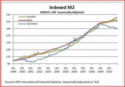
Their best argument has been “OK, but M2 fell sharply in the Great Depression, and M2 has risen briskly in this crisis.”  At that point I am usually stumped, and merely remind people that the profession no longer paid attention to M2 after the early 1980s, regarding it as “unreliable.”  But now I have a better answer.  I was reading a post by Justin Irving and came across this very interesting graph:

At first glance it doesn’t look like much of interest has happened to the eurozone money supply.  But remember that growth tends to be exponential, and so please visually follow the red euro M2 line upward.  Notice the break in growth in 2008.  Where would the money supply be if the ECB had maintained steady eurozone M2 growth?  Justin also supplied me with the actual seasonally adjusted data.  Here are some data points:

Date                                    M2          growth from 27 months earlier

April 2004                      5339999               14.9%

July 2006                       6372397              19.3%

October 2008                8014245              25.8%

January 2011                8413040                5.0%

So after rising at fairly rapid rates for years, M2 growth slows to barely over 2% annual rate over the past 27 months.  What would Milton Friedman say about that?

If pressed, Keynesians will usually point to real interest rates as the right measure of monetary ease or tightness.  By that criterion the Fed adopted an ultra-tight monetary policy in late 2008.  Monetarists will usually say that M2 is the best criteria for the stance of monetary policy.  By that criterion the ECB adopted an ultra-tight monetary policy in late 2008.  And yet it’s difficult to find a single prominent macroeconomist (Keynesian or monetarist) who has publicly called either Fed or ECB policy ultra-tight in recent years.  Maybe tight relative to what is needed, but not simply “tight.”

I’m calling out my profession.  Do they really believe what they claim to believe about good and bad indicators of monetary tightness?  Or in a crisis do they atavistically revert to the crudest measure of all, nominal rates.  Joan Robinson is famous for once having argued that easy money couldn’t possibly have caused the German hyperinflation, after all, nominal interest rates in Germany were not low during 1920-23.  Have we advanced at all beyond Joan Robinson in the 73 years since she made that infamous remark?  I used to think the answer was yes; now I’m not so sure.

[BTW, modern monetarists like Michael Belongia and William Barnett advocate use of a divisia index for money.  I saw a paper by Josh Hendrickson that showed by that measure money became very tight in the US during 2008.]

Justin’s post also contains another interesting idea.  Notice how much more slowly Danish M2 grew as compared to Swedish, or even eurozone M2.  Sweden has a floating exchange rate and devalued sharply in late 2008, Denmark’s currency is fixed to the euro, and Denmark’s economy is much weaker than Sweden’s (in terms of NGDP and RGDP growth.)  Here’s Justin:

I am examining this issue in my Masters Thesis and it just occurred to me that it might be interesting to see how Denmark and the ECB compare to Sweden on Milton Friedman’s favored measure of monetary policy-M2 growth.  M2 is a standard measure of how much money there is in the banking system of an economy.  It is beyond the point of this post, but there is good reason to think that if M2 drops precipitously, that spending will fall and that the economy will grow below its potential.  Unfortunately we cannot see M2 for Finland alone as there is no real way of distinguishing between the stock of Euros within the Finnish economy, and those in the broader world.  The Danish crown however is something like that radioactive dye physicians inject into peoples veins so that they can see the circulatory system on an x ray.  The Danish currency is essentially the Euro, except that we can track it by the fact that it has pictures of Viking longships on it if it is currency, or a DKK currency ID next to it if it is electronic money.

Because Denmark fixes the price of the Danish Crown in terms of Euro, the central bank is constrained in how it can stabilize M2.  Central banking is, at the end of the day, pretty simple (no to be confused with easy).  The only thing the bank can really do is change the quantity of money and see how the market reacts.  Most of the time, central banks pick an interest rate they think appropriate and print money or pull it from circulation (by selling financial assets or foreign currency they have accumulated) until the interest rates moves where they want it.  When interest rates fall to zero, central banks need to pick other variables to guide their money printing decisions, such as stocks, exchange rates, consumer prices or nominal GDP.  In the case of Denmark, the central bank targets the exchange rate against the Euro by buying and selling the Danish crown in currency markets so that its rate against the Euro never changes.  As Denmark is an open economy with free capital flow, this means that they have essentially no control over their monetary policy.  Danish interest rates and money supply have to adjust to whatever is necessary to keep the Euro rate stable.

I love Justin’s radioactive dye analogy; it reminded me of something I noticed in the Great Depression.  In the US the monetary base fell 7% between October 1929 and October 1930, under the Fed’s tight money policy.  Then it rose substantially after October 1930.  But money didn’t become easier, rather the Fed was partially accommodating the hoarding of cash and reserves during banking panics.  But not fully accommodating the demand, as NGDP continued falling sharply after October 1930.  How could we know if this explanation is correct?  One answer would be to look for a similar economy, without banking panics.  In Canada there were no bank panics, and cash in circulation continued falling throughout 1929-32, if my memory is correct.  Because the US deflation was transferred to Canada via the international gold standard, they had no choice but to deflate their own currency.  Canada in the early 1930s is like Denmark in the past three years.

There’s an old fairy tale where a beautiful princess looks in the mirror and sees her true self, which looks more like an ugly witch.  The US monetary policy looked beautiful in the early 1930s, if one just focused on the base.  But all one had to do was look to the north to see just how ugly it really was.  If the ECB wants to take a look in the mirror, I suggest they take a look at the contrast between Swedish and Danish M2 growth.  The Danish policy it what their policy really looks like.  It’s not a pretty sight.

BTW, Justin’s blog post is more valuable than most master’s theses that I have seen.

PS.  I believe Canada may have done a small devaluation in late 1931, but not enough to prevent deflation.

There has been a recent upswing in conservative articles discussing the idea of going back to some sort of gold standard.  I don’t think people realize how dangerous this idea is.  You can’t just “give it a shot” and see how it works out.  It’s like marrying the daughter of a Mafia chieftain–you need to be very sure you are willing to commit.

A true gold standard (not Bretton Woods) allows Americans to buy or sell gold.  If you are not 100% committed to staying on gold, but instead hint you might devalue the dollar at some point, people will dump dollars and buy gold.  The increase in demand for gold will raise its value, or purchasing power.  This is deflationary under a gold standard, where the nominal price of gold is fixed.

Nor is this merely a theoretical problem.  There were large bouts of private gold hoarding during four periods of the Great Depression, all associated with devaluation fears; the last half of 1931, spring 1932, February 1933, and late 1937.  All four were associated with economic distress, falling stock and commodity prices, etc.  And there is event studies-type evidence showing causation going from gold hoarding to deflation.

It’s not easy to know which price of gold would be appropriate.  Perhaps market gold prices would go to the right level after an “announcement” of a return to gold, but even that depends on the announcement being 100% credible.  But after you re-peg, the real value of gold can change due to industrial demand shifts, even if there is no monetary hoarding of gold.  Furthermore, all countries are not likely to follow the US back on gold, so you might have monetary gold hoarding in Europe, as people feared for the euro.  Booming Asia might increase the industrial demand for gold, just as it has raised the demand for many other metals.

And there is little room for error.  A 10% increase or decrease in the real value of gold seems very small when it is just a commodity.  But under a gold standard that sort of shift can be accommodated only by changing the overall price level by 10%.  A sudden 10% rise or fall in the price level is very destabilizing to the economy.

Even if the government is committed to gold, investors may fear the next government won’t be (remember FDR?)  In that case the promise to stay on gold may not be credible.  In the old days there was a powerful emotional attachment to gold, as paper money was feared as inevitably leading to hyperinflation.  Only then will voters be willing to suffer austerity to stay on gold.  A modern analogy is the long painful struggle of Argentina to stay on its currency board during the 1998-2001 deflation, attributable to a fear they would return to hyperinflation.  But we now know that fiat money can produce modest inflation rates, so our voters won’t undergo the pain of the mid-1890s, or early 1930s, just to stay on gold.  And if you aren’t willing to undergo that pain, the system won’t work.

Some supporters point to Bretton Woods, but that “worked” in direct proportion to the extent that the gold constraints were ignored.  Gold was highly overvalued after the 1933 devaluation, and then the US grabbed a huge share of the world’s gold in the run-up to WWII.  After the war those two factors gave us an unprecedented amount of slack, where we could mildly inflate until gold was no longer overvalued.  Once we reached that point in the late 1960s, the system immediately fell apart.  It would have collapsed even sooner if Americans had been allowed to own gold.  And if LBJ had tried to deflate to stay on gold, Americans (if allowed to) would have hoarded gold in the (correct) expectation that the next president would devalue the dollar, putting expediency ahead of principle.  That hoarding would have had the same effect as the hoarding of the early 1930s–deflation and depression.

HT:  Bruce Bartlett

PS:  Today’s NYT said:

Economists are now engaged in a spirited debate, much of it conducted on popular blogs like Marginal Revolution, about the causes of the American jobs slump. Lawrence Katz, a Harvard labor economist, calls the full picture “genuinely puzzling.”

If you check the four links you won’t find me, but the link to MR (Alex Tabarrok) starts as follows:

I find myself in the unusual position of being closer to Paul Krugman (and Scott Sumner, less surprising) than Tyler on the question of Zero Marginal Product workers.

Close, but no cigar.  Still I guess it’s progress being just “one degree of separation” away from the Times.