Money and Inflation, Pt 3 (The Quantity Theory of Money and the Great Inflation)
Here’s my Russ Roberts Podcast. Patrick sent me my AEI presentation and my Larry Kudlow interview (67 minute mark, 3/23/13).
There are two aspects of fiat money that make the supply and demand for a fiat currency differ from the commodity money model:
1. The government has almost unlimited control over the stock of currency, and can produce currency at near zero cost.
2. The demand for money becomes unit elastic, in response to changes in the value of money (1/P).
Here’s how the money supply and demand graph looks for fiat currency:
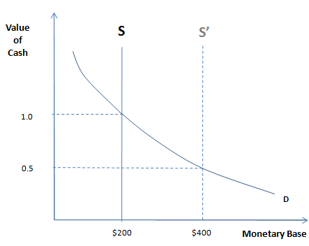
Monetary policy has switched from influencing the demand for the MOA (under the gold standard), to a policy of influencing the supply of the MOA (although money demand is also affected by Fed policies.) The Fed can shift the supply curve to the left or right via open market operations or discount loans. Thus the “supply curve” is actually a policy tool, representing the quantity of base money.
In the past I used to teach the quantity theory of money with a “helicopter drop” example, but I now see that won’t work—people get the wrong message. Traditional OMOs also confuse people. More specifically:
1. Some Keynesians believe it matters a lot whether the currency is introduced via a “helicopter drop” or OMOs. The term ‘helicopter drop’ actually refers to combined monetary/fiscal expansion. Money dropped out of helicopters is sort of like “welfare” payments, and it’s also an expansion of the money stock. So it’s like paying for a new entitlement program by printing cash and spending it. But these Keynesians are wrong. The fiscal effects are utterly trivial as compared to the monetary effect, at least during normal times. Increasing the base by 0.2% of GDP during normal times is a big deal. Increasing debt held by the public by 0.2% hardly matters at all.
2. Some Austrians worry about “Cantillon effects,” which means they think it’s important to consider who gets the money first. (Although the term also has other meanings). They assume that that lucky group will boost its spending. Yet the money is not given away, it’s sold at market prices. So the person getting the money first is not significantly better off, and hence has little incentive to buy more real goods and services.
Both errors share something in common—the notion that money injections matter because “people with more money will spend more.” But this subtly confuses wealth and money. In everyday speech we might say; “a billionaire buys a big yacht, because he has lots of money.” But we really mean he has lots of wealth. The billionaire might have very little cash. So if we are truly going to understand the pure effects of monetary injections (without fiscal or Cantillon effects), we have to consider a form of injection that doesn’t appear to make anyone “better off,” so that people would have no obvious reason to go out and buy more stuff.
I’d like to assume that money is injected according to the following formula: Suppose there are 100 million Americans that get substantial checks from the government each year (more than $200). These include tax rebates, veterans benefits, unemployment insurance, government worker salaries, Social Security, etc. A cross section of America. The Fed wants to increase the base by $20 billion this year. Have the Treasury pay each of the 100 million Federal check recipients the first $200 due to them in cash, and the rest by check. In this case people are not getting any additional money, it’s just that some of it comes in the form of cash rather than the usual checks. If the Fed had decided not to increase the base, the extra $200 would have been paid by check. That is the essence of monetary policy, with no distracting bells and whistles.
People don’t want to hold that much extra cash, so they’ll get rid of it. But how? Obviously not by burning it. Now we come to the concept that lies at the heart of money/macro—the fallacy of composition. Individuals can get rid of the cash they don’t want, but society as a whole cannot, at least not in nominal terms. How do we reconcile that seeming paradox?
Take an example where the Fed doubles the currency stock, from $200 to $400 per capita (shown in the graph.) How do we reach a new equilibrium? In the short run prices are sticky, and short term interest rates might fall. But over time prices will adjust, and the public will reach a new equilibrium where they are happy holding $400 per capita. How much do prices have to rise for supply to equal demand at the original interest rate?
If we assume that people care about purchasing power rather than nominal quantities, then prices must double, so that the purchasing power of the stock of cash returns to its original level. Say that people used to hold enough cash to make one week’s worth of purchases ($200.) Then prices must rise until one week’s worth of purchases costs $400. In other words prices rise in proportion to the rise in the currency stock. And that means the demand curve for the MOA is unit elastic. In contrast, when silver (or gold) was the MOA, the demand for those assets was not unit elastic. Currency is special. Its only value is its purchasing power—it has no industrial uses at all (unlike gold.)
The assumption of a unit elastic demand for currency leads to the Quantity Theory of Money. If you double the money supply, the value of money will fall in half, and the price level will double. Of course this assumes the demand for money does not change over time. But money demand does change. It would be more accurate to say; “a change in the money supply causes the price level to rise in proportion, compared to where it would be if the money supply had not changed.” But even that’s not quite right because (expected) changes in the value of money can cause changes in the demand for money. So all we can really say is:
One time changes in the supply of money cause a proportionate rise in the price level in the long run, as compared to where the price level would have been had the money supply not changed.
That’s because one time changes in the money supply probably don’t shift the real demand for money in the long run. This is a somewhat weaker version of the QTM, but is the most defensible version. In my view the QTM is most useful when there are large changes in the supply of money, and/or over the very long run. Especially when there are large changes in the supply of money, year after year, over a very long period of time. In other words, international data over a long period during the global Great Inflation. Robert Barro’s macro text (4th ed.) has the perfect data set for thinking about the QTM; 83 countries, over roughly 30 years, when inflation rates were very high and varied dramatically from one country to another. Here are the top 10 and the bottom 10 on the list:
Country MB growth RGDP growth Inflation Time period
Brazil 77.4% 5.6% 77.8% 1963-90
Argentina 72.8% 2.1% 76.0% 1952-90
Bolivia 49.0% 3.3% 48.0% 1950-89
Peru 49.7% 3.0% 47.6% 1960-89
Uruguay 42.4% 1.5% 43.1% 1960-89
Chile 47.3% 3.1% 42.2% 1960-90
Yugoslavia 38.7% 8.7% (FWIW) 31.7% 1961-89
Zaire 29.8% 2.4% 30.0% 1963-86
Israel 31.0% 6.7% 29.4% 1950-90
Sierra Leone 20.7% 3.1% 21.5% 1963-88
. . .
Canada 8.1% 4.2% 4.6% 1950-90
Austria 7.1% 3.9% 4.5% 1950-90
Cyprus 10.5% 5.2% 4.5% 1960-90
Netherlands 6.4% 3.7% 4.2% 1950-89
U.S. 5.7% 3.1% 4.2% 1950-90
Belgium 4.0% 3.3% 4.1% 1950-89
Malta 9.6% 6.2% 3.6% 1960-88
Singapore 10.8% 8.1% 3.6% 1963-89
Switzerland 4.6% 3.1% 3.2% 1950-90
W. Germany 7.0% 4.1% 3.0% 1953-90
Homework for today:
Answer the following 5 questions and you’ll understand the QTM:
1. Does the “eyeball test” provide more support for the QTM in the low or the high inflation countries? What does this tell us about its actual applicability to each group? How does its relative applicability to each group depend on which of the definitions of the QTM (discussed above) is used?
2. In 71 of the 83 countries the money growth rate exceeds inflation, and in 12 the inflation rate exceeds the money growth rate. Explain why the ratio is so lopsided.
3. The gap between money growth rates and inflation exceeds 10% in only one of the 83 countries (Libya–not shown.) Why does the gap rarely exceed 10%?
4. Do most of the twelve cases where inflation exceeds money growth occur in low or high inflation countries. Explain why.
5. Explain what sort of inflation data would better explain the gap: average inflation rates, the change in the inflation rate, or changes in the expected inflation rate.
I’ll answer tomorrow in the next post. The commenter with the best set of answers gets a gold star.