In a recent post, I quoted from a Josh Hendrickson review of The Midas Paradox, particularly the discussion of the deflationary impact of devaluation fears during the 1930s.  I viewed this as a bit of a puzzle.  It’s no surprise that devaluation expectations would raise the demand for gold, and hence the value of gold.  And since gold was a medium of account, that would be deflationary.  But it would also reduce the demand for currency, which was also a medium of account. So why didn’t it reduce the value of currency?  After all, an actual devaluation would reduce the value of currency.

Bob Murphy has a very interesting explanation in the comment section:

Scott,

Forgive me if I’m just saying the same thing you did, in different vocabulary, but, wouldn’t the following make sense? I don’t see what the mystery here is.

(1) Right now the US government will trade gold for dollars at $20.67 / ounce.

(2) Investors are worried that next year, they will charge people $35 to give them an ounce of gold.

(3) So investors naturally shift out of dollars and into gold. (Just like if you suddenly thought Acme stock would go from $20.67 today to $35 next year, at a time of very low interest rates, you would rebalance your portfolio to buy more Acme stock than you were holding 5 minutes ago.)

(4) Yet since right now the US is still on the gold standard at $20.67, as people try to get rid of dollars and hold more gold, the only way to maintain that rate is for the US Treasury to absorb dollars and release gold from its vaults.

(5) As the total amount of dollars held by the public shrinks, prices in general (quoted in dollars) fall.

Am I missing something?

That may indeed be the solution.  If so, what did I overlook?

1. Perhaps I focused too much on the actual currency stock, which did not tend to fall during these episodes.  But that may be because devaluation fears were associated with banking crises.

2.  So let’s assume that Bob is correct that devaluation fears are deflationary because they reduce the currency stock, ceteris paribus.  In that case, the banking panics that increased currency demand could be viewed as a second deflationary shock, and perhaps the central bank increased the currency stock enough to partially offset this increase in currency demand, but not the initial shock of more demand for gold.

3.  Suppose there had been no banking panics.  And suppose that the central bank responded to fears of devaluation by preventing the money stock from falling. What then?  In that case, the shock might not have been deflationary.  But that’s not because devaluation fears are not deflationary, but rather because the central bank would have taken an expansionary monetary action to offset the private gold hoarding.  Under a gold standard, an outflow of gold into private hoards should normally result in a smaller currency stock, keeping the ratio of gold to currency stable.  So if the central bank refuses to let the currency stock fall, that’s an expansionary monetary policy.  It wouldn’t mean the devaluation fears were not deflationary, ceteris paribus, but rather that the deflationary impact of one shock was being offset by an expansionary policy elsewhere.

4.  Bob mentions that the M1 money supply did fall during the banking panics, which simplifies things, but I prefer to do all the analysis through the currency stock (or monetary base), which in this case made things more complicated for me.

5.  How about from a finance perspective?  At first glance it seems weird that people would hold both gold and currency, even though the expected return on gold was higher during a period of devaluation fears.  But gold and currency may not be perfect substitutes, and as the stock of currency declines the marginal liquidity services it provides increase relative to gold.  Or perhaps those who feared devaluation correctly anticipated that the government would confiscate domestic gold hoards.

I am still a bit confused by the evidence that markets respond differently when devaluation (or revaluation) seems imminent.  The markets were not adversely affected by the gold crisis in early March 1933, anticipating that FDR would soon do something dramatic.  And they were adversely affected by fears of revaluation during the “gold panic” of 1937.  So there are still some unresolved puzzles in my mind.  But Bob’s explanation for the basic pattern of the early 1930s seems better than anything else I’ve seen.

PS.  I am currently in San Diego, at the Western Economic Association conference. Blogging will be sporadic for most of the summer.

Josh Hendrickson has a very good review of my Great Depression book, published in the Journal of Economic History.  Here is one part of the review:

The role of monetary policy expectations is central to the modern New Keynesian model. Forward guidance has been a tool of monetary policy in the aftermath of the Great Recession. The role of expectations following the increase in the price of gold would seem to provide some empirical support for both the model and the practice. However, hidden in Sumner’s book is a cautionary tale about this type of policy. While it is true that the price level increased immediately following the increase in the price of gold, the gold standard has a built-in mechanism, namely international price arbitrage, which ensures that the price level would eventually rise. In a modern fiat regime there is no automatic mechanism capable of generating this outcome. The public’s expectations in a fiat regime depend on the commitment of the central bank to do something in the future. This word of caution is important because a key and recurring empirical observation in Sumner’s book is that fears of devaluation often led to private gold hoarding, which was deflationary (precisely the opposite effect of an actual devaluation). Sumner leaves the question of why expectations of devaluation and actual devaluation had precisely the opposite effect as a subject for future research. However, one possible hypothesis is that an actual devaluation had a built-in commitment mechanism. At the very least, this should give current policymakers some pause about forward guidance.

I think Josh is correct about the commitment mechanism, which is what made the 1933 dollar depreciation so effective.  Josh is right that I struggled with explaining why expectations of devaluation were often contractionary (not just in the Depression, BTW, but also in the 1890s.) It may have something to do with the dual media of account, gold and currency.  In a modern fiat money system, there is only one medium of account—base money.  If there is a 2% chance that the dollar will be devalued by 50% next year, then the expectation is that gold will earn a return 1% higher than currency.  If government bonds are also earning near zero interest rates, then gold becomes an relatively attractive investment.  This drives up the real value of gold all over the world, including the country where devaluation is thought to be a possibility.  That’s deflationary.  On the other hand, this reduces the demand for currency, which should be inflationary. And until the devaluation actually occurs, currency is pegged to gold at a fixed price.  There may be a way to model all this, but it’s not clear to me what it is.

An added complication is that fear of devaluation also seemed to trigger bank runs during 1931-33, and that’s also a deflationary factor.

Rajat asked one of his characteristically probing questions, in the previous post:

As you’ve often said with monetary policy, it all depends on the yardstick or counterfactual. With your examples, because you’ve put the focus on interest rates, the reader naturally assumes that the counterfactual is no change in official interest rates. For example, in (1), surely the cut in the Fed Funds rate from 5.25% to 2% was less contractionary than if the Fed did not lower the rate? The money supply may not have risen in 2007-08, but wouldn’t it have fallen if rates were kept at 5.25%, as the market devoured the short-term securities the Fed offered at that yield? I understand that the reduction in official rates was not expansionary in any meaningful sense (ie against a benchmark of ideal monetary policy under inflation or NGDP targeting).

This is probably correct, but I’d argue that it could also be misleading, resulting in too much reassurance that interest rates aren’t that bad an indicator after all.  Rajat’s point is that if the Fed never even began cutting rates, then they would have had to reduce the money supply rather dramatically.  So much so that NGDP would have done even worse than with cut from 5.25% to 2.0%.  So does that mean the interest rate cut was expansionary after all?  Not quite.

Consider the two following hypotheticals:

A.  No change in the base from August 2007 to May 2008, rates fall from 5.25% to 2.0% (actual policy)

B.  The base rises by 5%, while rates move from 5.25% in August 2007 to 5.25% in May 2008.

I would claim that policy B is almost certainly more expansionary.  Rajat might reply that policy B was not an option.  If the monetary base had risen by 5%, then interest rates would have declined even more rapidly than they actually did.

I don’t quite agree, although for any given day I’d agree with that claim.  Thus on any given day, a lower fed funds target requires a larger base than otherwise (at least before IOR was instituted in October 2008).  But that true fact leads many Keynesians to jump to a seemingly similar, but unjustified conclusion.  Many people assume that over a 9-month period a more expansionary monetary policy implies a faster decline in interest rates.

In fact, option B probably was available to the Fed, but only if they moved much more aggressively in the early part of this period and/or if they changed their policy target.  Thus there are two possible ways the Fed might have achieved policy option B:

B1.  Cut rates sharply enough in August 2007 to dramatically boost NGDP growth expectations, and then gradually raise rates enough over the next few months to get them back to 5.25% by May 2008.  In that case, NGDP growth would have held up well, and yet the path of interest rates over that period would have ended up higher than otherwise.

B2.  Adopt a policy of 5% NGDPLT, which would have radically changed expectations, and hence boosted the Wicksellian equilibrium rate.

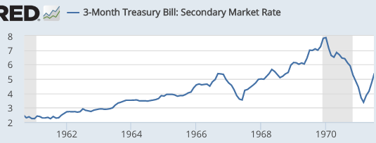
Rajat might view option B2 as cheating, so let me make a case for option B1.  I’d argue that the Fed did almost exactly what I describe in option B1 during 1967.  Just to set the scene, the economy was slowing sharply during early 1967, and some people worried that we might enter a recession.  The Fed moved quite aggressively, and their move was so successful that over a period of 10 months there was no rate cut at all.

3 month T-bill yields:

January 1967:  4.72%

June 1967:  3.54%

November 1967:  4.73%

So interest rates were basically unchanged over this period, and yet I’d argue that policy was far more expansionary than during August 2007 to May 2008, when rates fell sharply.  The monetary base grew by over 5% in just 10 months, and this allowed the US to avoid recession.

(BTW, in retrospect, a mild recession would have been preferable in 1967, as a way of avoiding the Great Inflation.  Instead, the US left the gold standard in April 1968, Bretton Woods blew up 3 years later, and the rest is history.  But since policymakers didn’t know all of this would occur, the mistake of the 1960s was sort of inevitable—just a question of when.)

In 1967, the expansionary policy early in the year boosted NGDP growth expectations enough so that they could raise rates back up later in the year, and still see robust NGDP growth.  In 1968, interest rates rose still higher, but this was expansionary because the base was also rising briskly.  So you have both rising base velocity (from higher rates) and a rising monetary base.

There’s a grain of truth in Rajat’s comment, but it’s best thought of as applying to a given day, where a lower interest rate implies a faster growth in the money supply, and easier money.  Over a more extended period of time things become much dicier.  Those who focus on interest rates are more likely to be led astray, the longer the period being examined.

Here’s Nick Rowe:

I understand how monetary policy would work in that imaginary Canada (at least, I think I do). Increasing the quantity of money (holding the interest rate paid on money constant) shifts the LM curve to the right/down. Increasing the rate of interest paid on holding money (holding the quantity of money constant) shifts the LM curve left/up. Done.

It’s a crude model of an artificial economy. But it’s a helluva lot better than a simple New Keynesian model where money (allegedly) does not exist and the central bank (somehow) sets “the” nominal interest rate (on what?).

I think this is right.  But readers might want more information.  Exactly what goes wrong if you ignore money, and just focus on interest rates?  Let’s create a simple model of NGDP determination, where i is the market interest rate and IOR is the rate paid on base money:

MB x V(i – IOR) = NGDP

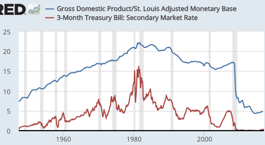
In plain English, NGDP is precisely equal to the monetary base time base velocity, and base velocity depends on the difference between market interest rates and the rate of interest on reserves, among other things.  To make things simple, I’m going to assume IOR equals zero, and use real world examples from the period where that was the case.  Keep in mind that velocity also depends on other factors, such as technology, reserve requirements, etc., etc.  The following graph shows that nominal interest rates (red) are positively correlated with base velocity (blue), but the correlation is far from perfect.

[After 2008, the opportunity cost of holding reserves (i – IOR) was slightly lower than shown on the graph, but not much different.]

What can we learn from this model?

1.  Ceteris paribus, an increase in the base tends to increase NGDP.

2.  Ceteris paribus, an increase in the nominal interest rate (i) tends to increase NGDP.

Of course, Keynesians often argue that an increase in interest rates is contractionary.  Why do they say this?  If asked, they’d probably defend the assertion as follows:

“When I say higher interest rates are contractionary, I mean higher rates that are caused by the Fed.  And that requires either a cut in the monetary base, or an increase in IOR.  In either case the direct effect of the monetary action on the base or IOR is more contractionary than the indirect effect of higher market rates on velocity is expansionary.”

And that’s true, but there’s still a problem here.  When looking at real world data, they often focus on the interest rate and then ignore what’s going on with the money supply—and that gets them into trouble.  Here are three examples of “bad Keynesian analysis”:

1. Keynesians tended to assume that the Fed was easing policy between August 2007 and May 2008, because they cut interest rates from 5.25% to 2%.  But we’ve already seen that a cut in interest rates is contractionary, ceteris paribus. To claim it’s expansionary, they’d have to show that it was accompanied by an increase in the monetary base.  But it was not—the base did not increase—hence the action was contractionary.  That’s a really serious mistake.

2.  Between October 1929 and October 1930, the Fed reduced short-term rates from 6.0% to 2.5%.  Keynesians (or their equivalent back then) assumed monetary policy was expansionary.  But in fact the reduction in interest rates was contractionary.  Even worse, the monetary base also declined, by 7.2%.  NGDP decline even more sharply, as it was pushed lower by both declining MB and falling interest rates.  That’s a really serious mistake.

3.  During the 1972-81 period, the monetary base growth rate soared much higher than usual.  This caused higher inflation and higher nominal interest rates, which caused base velocity to also rise, as you can see on the graph above.  Keynesians wrongly assumed that higher interest rates were a tight money policy, particularly during 1979-81.  But in fact it was easy money, with NGDP growth peaking at 19.2% in a six-month period during late 1980 and early 1981.  That was a really serious error.

To summarize, looking at monetary policy in terms of interest rates isn’t just wrong, it’s a serious error that has caused great damage to our economy.  We need to stop talking about the stance of policy in terms of interest rates, and instead focus on M*V expectations, i.e. nominal GDP growth expectations.  Only then can we avoid the sorts of policy errors that created the Great Depression, the Great Inflation and the Great Recession.

PS.  Of course Neo-Fisherians make the opposite mistake, forgetting that a rise in interest rates is often accompanied by a fall in the money supply, and hence one cannot assume that higher interest rates are easier money.  Both Keynesians and Neo-Fisherians tend to “reason from a price change”, ignoring the thing that caused the price change.  The only difference is that they implicitly make the opposite assumption about what’s going on in the background with the money supply. Although the Neo-Fisherian model is widely viewed as less prestigious than the Keynesian model, it’s actually a less egregious example of reasoning from a price change, as higher market interest rates really are expansionary, ceteris paribus.

PPS.  Monetary policy is central bank actions that impact the supply and demand for base money.  In the past they impacted the supply through OMOs and discount loans, and the demand through reserve requirements.  Since 2008 they also impact demand through changes in IOR.  Thus they have 4 basic policy tools, two for base supply and two for base demand.

PPPS.  Today interest rates and IOR often move almost one for one, so the analysis is less clear.  Another complication is that IOR is paid on reserves, but not currency.  Higher rates in 2017 might be expected to boost currency velocity, but not reserve velocity.  And of course we don’t know what will happen to the size of the base in 2017.

One of the ways that macro differs from micro is that macro is essentially a branch of history.  Micro is not.  And yet today’s macroeconomists often have not studied monetary history.  Marcus Nunes and Ramesh Ponnuru directed me to a paper by White House economics advisor Jason Furman:

A decade ago, the prevalent view about fiscal policy among academic economists could be summarized in four admittedly stylized principles:

1. Discretionary fiscal policy is dominated by monetary policy as a stabilization tool because of lags in the application, impact, and removal of discretionary fiscal stimulus.

2. Even if policymakers get the timing right, discretionary fiscal stimulus would be somewhere between completely ineffective (the Ricardian view) or somewhat ineffective with bad side effects (higher interest rates and crowding-out of private investment).

3. Moreover, fiscal stabilization needs to be undertaken with trepidation, if at all, because the biggest fiscal policy priority should be the long-run fiscal balance.

4. Policymakers foolish enough to ignore (1) through (3) should at least make sure that any fiscal stimulus is very short-run, including pulling demand forward, to support the economy before monetary policy stimulus fully kicks in while minimizing harmful side effects and long-run fiscal harm.

Today, the tide of expert opinion is shifting the other way from this “Old View,” to almost the opposite view on all four points.

I think this is right, but where Furman and I differ is on the desirability of this shift.

Furman refers to the view “a decade ago” but he might just as well have said 90 years ago.  The New Keynesian consensus is actually not all that far from the views of progressive economists back in the 1920s, which favored a price level target and were skeptical about fiscal policy.  After the 1930s, opinions moved in the old Keynesian direction.  It wasn’t until the 1960s that the tide started swinging away from the “vulgar Keynesian” view that fiscal policy was more important than monetary policy.  Friedman and Schwartz started he counterrevolution, and by the 1990s it was pretty much complete.  Stabilization policy should rely on monetary policy.

And now we have still another swing of the pendulum, back toward the old Keynesian views of the post-1936 period. Here’s Furman:

The New View of fiscal policy largely reverses the four principles of the Old View—and adds a bonus one. In stylized form, the five principles of this view are:

1. Fiscal policy is often beneficial for effective countercyclical policy as a complement to monetary policy.

2. Discretionary fiscal stimulus can be very effective and in some circumstances can even crowd in private investment. To the degree that it leads to higher interest rates, that may be a plus, not a minus.

3. Fiscal space is larger than generally appreciated because stimulus may pay for itself or may have a lower cost than headline estimates would suggest; countries have more space today than in the past; and stimulus can be combined with longer-term consolidation. 

4. More sustained stimulus, especially if it is in the form of effectively targeted investments that expand aggregate supply, may be desirable in many contexts.

5. There may be larger benefits to undertaking coordinated fiscal action across countries.

Those old Keynesian views of the late 1930s were rejected for lots of good reasons.

I’m not quite sure what is more humiliating for the profession of macroeconomics:

1.  That we keep making the same mistakes, over and over again.

2.  That we change our views of macro on “new information”, which in fact is not new to anyone with an even passing interest in macro history.  (I.e., who know that the temporary QE of 1932 had little impact, just as the more recent temporary QE had little effect.)

3.  That we don’t pay attention to the empirical studies that refute old Keynesianism.

4.  That many macroeconomists are not even aware of the cyclical nature of their field.

It’s not unusual to find this sort of cyclicality in the arts.  For instance, in the arts there are swings back and forth between a more “classic” style and a more “romantic” style.  But it’s kind of embarrassing to see this in a science.

(And don’t embarrass yourself by arguing macroeconomics is not a science.  Of course it’s a science.  It’s failed science, but then so are some of the other sciences, at least based on what I’ve read about the crisis in replication.  The term ‘science’ is not a compliment, it’s not some sort of award given to a field, like a Nobel Prize.  It’s simply a descriptive term for a field that builds models that try to explain how the world works.  Saying that science must be successful to be viewed as science is as silly as saying that a work of art must be good to be considered art.)

We need a “timeless” macro.  That is, theories should not be developed to meet the specific conditions in the economy, at that moment.  And yet that’s exactly what old Keynesianism is, which is why it goes in and out of style.  Instead, theories should be developed to explain the entire history of macroeconomics—the full data set.  If your model is not good at explaining hyperinflation, stagflation, liquidity traps and the Great Moderation, then it’s not a good theory.

Old Keynesianism is not a good theory.

PS. I’d like to congratulate Ben Klutsey for winning the Great Communicators Tournament in Washington DC on Wednesday night. Some of you may know that David Beckworth and I both participate in the Mercatus Center’s Program on Monetary Policy. Unfortunately we both live some distance from the headquarters in Arlington, VA. Ben is the program’s manager, and does a lot of the behind the scenes work that readers might not be aware of. I feel lucky to work with someone who is both a very nice guy and a highly talented manager.

Also congratulations to runner-up Charles Blatz, another Mercatus employee.