Archive for the Category Monetary Theory


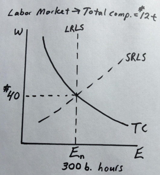
Are recessions about employment?

I’d say yes, but Nick Rowe disagrees.  He recently tweeted an old post from 2015, which ends as follows:

Recessions are not about output and employment and saving and investment and borrowing and lending and interest rates and time and uncertainty. The only essential things are a decline in monetary exchange caused by an excess demand for the medium of exchange. Everything else is just embroidery.

First I’m going to tell you why I disagree, and then I’ll explain why my disagreement is not very important, at least for the US economy.

I don’t believe that terms like “monetary exchange” and “excess demand” are clearly defined.  In my view, the most useful definition of a recession is a slowdown in employment growth that is sudden, significant and in some sense “anomalous”.  By that I mean a slowdown in employment growth that seems unrelated to fundamental factors such as demographics or preferences.

As this graph shows, slowdowns in employment growth are extremely strongly correlated with “recessions”, as defined by the NBER.   (The end of WWII was a bit weird. But that was an unusual period, with women entering the labor force during the war, then leaving, and soldiers returning home.)

Screen Shot 2019-01-20 at 4.42.40 PM

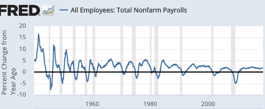
Thus in an accounting sense, recessions are mostly about employment, not factors such as productivity.  And most economists believe the reduction in employment during recessions is non-optimal, that it does not reflect preferences.  So what causes this slowdown?

In my view (and I think Nick agrees), these recessions are caused by sharp declines in NGDP growth in an economy with sticky wages and prices.  Here is some data on NGDP growth:

Screen Shot 2019-01-20 at 4.39.07 PM
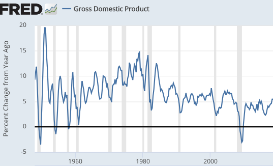
Once again, the correlation is quite strong.  At the same time, I could easily imagine other factors causing a recession.  A government might institute an extremely high minimum wage rate, and then later remove this wage floor.  This would temporarily depress employment growth, without impacting NGDP.  So I don’t see how recessions can always be caused by an excess demand for money, unless they are defined that way.  But since we cannot directly measure excess money demand, that’s not a useful definition.  All we can do is look at various macro variables and infer that there was an excess demand for money.

Nor can we solve the problem by looking at the other part of Nick’s definition, a “decline in monetary exchange”.  If monetary exchange suddenly falls in half, and all wages and prices are cut in half by administrative fiat, there may not be a recession.  Indeed something like this occurs during a currency reform.

[Please don’t misinterpret this observation.  I am not claiming that making wages and prices flexible is a good way of avoiding recessions, it isn’t.  Rather the thought experiment shows that a recession is not identical to a decline in monetary exchange.  And keep in mind that NGDP is only a tiny fraction of “monetary exchange”, which is dominated by the exchange of money in the financial markets.]

Let’s look at the recession that is generally regarded as the least monetary of all post-WWII US recessions, November 1973 to March 1975:

Screen Shot 2019-01-20 at 4.38.19 PM
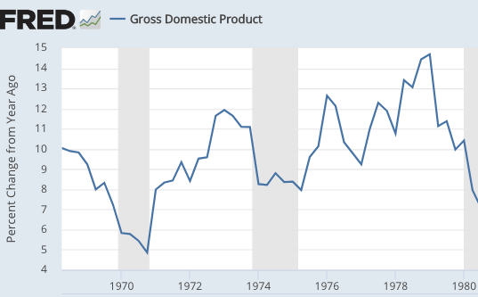
That graph is actually pretty good for Nick’s claim, as even the least monetary of all recessions looks quite monetary.  NGDP growth slowed significantly during the 1974 recession.

On closer inspection, we can see why this is viewed as the least monetary recession.  The slowdown in NGDP growth was fairly mild compared to other recessions, whereas the fall in employment growth and RGDP was relatively severe, at least for the post-1965 period.

Many economists would attribute this to 1974 being an adverse “supply shock”, caused by soaring oil prices.  I’m not so sure, as the equally severe 1979-80 oil shock produced a boringly normal recession; that double-dip recession was about as severe as one would expect from the size of the NGDP growth slowdown in early 1980, and then again in 1981-82.  So even that double-dip “oil shock” recession looks quite monetary.

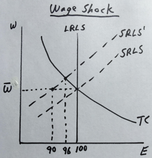
Instead, I believe the unusual severity of the 1974 recession reflects a “wage shock” caused by the removal of wage controls.  These same controls had artificially boosted output during 1972 (when Nixon just happened to be running for re-election), and we paid the price in 1974 (when Nixon was fittingly removed from office.)  As a result, wage growth actually rose during the 1974 recession.

Screen Shot 2019-01-20 at 6.40.44 PM

Rather than define a recession as a negative monetary shock that causes less monetary exchange, I’d rather say that a recession is a sudden, sizable, and anomalous slowdown in employment growth.  And then I’d say that US recessions are virtually always caused by monetary shocks that reduce NGDP growth, but in other countries (such as Venezuela and Zimbabwe) recessions are often caused by real shocks–usually bad (interventionist) government policies.

PS.  I understand that the correlation between NGDP and recessions doesn’t prove causation, but we have a mountain of other evidence suggesting that causation goes from monetary variables such as NGDP to employment.

We need to unify monetary theory and monetary policy

Before today’s post, a few quick comments.  I have a piece on Trump’s “deregulation” policies at MarketWatch.  I have a Ted talk on public opinion at Econlog.

It’s clear to me that there is something seriously wrong with the field of monetary economics.  The profession got 2008-09 almost entirely wrong.  But it’s hard to pin down exactly where the problem lies.  After all, there are increasingly sophisticated models being developed by economists who are much smarter than me.  These models feature rational expectations, and all the other bells and whistles you might want. I regret their focus on interest rates and inflation, but that doesn’t fully explain the problem.  While I prefer to talk about money and NGDP, anything that I believe can be translated into New Keynesianism by referring to the gap between the natural rate of interest and the market rate.  So where’s the problem?

In my view, the problem lies in the interface between sophisticated theoretical models and a very crude discourse on monetary policy.  This monetary policy discourse is little changed from 90 years ago, and not at all informed by recent developments in theory.

John Hall directed me to a James Hamilton post that included this remark:

Zhang’s suggested solution begins with the observation by Gurkaynak, Sack and Swanson (2005) that the news revealed by a typical FOMC announcement is multidimensional. The Fed is typically both changing the current interest rate and signaling the changes that are in store for the future.

Here’s my hypothesis.  Monetary models suggest that monetary policy actions are multidimensional, while most of the discourse on real world monetary policy treats policy as one dimensional—easier or tighter money, lying along a single line.  This has led to the confusing debate between Keynesians and NeoFisherians, which I’ll return to later.

Once monetary theorists understood that monetary policy actions affected the entire future path of policy, the modeling problem became more difficult.  At this point they should have stopped basing their models on interest rates, as this variable creates all sorts of indeterminacy issues, or perhaps I should say makes these issues even harder to grapple with—they can also occur when using money itself.

To make things simpler, I’m going to boil the multidimensional theoretical models down to two dimensions—levels and growth rates.  Obviously things are more complicated than that, but it’s enough to make my point about the disconnect between monetary theory and the modern discourse on monetary policy.  I’m also going to work with some alternative monetary instruments, that is, alternatives to interest rates.

Let’s start with the monetary base.  Any change in monetary policy has two dimensions, a level shift and a growth rate shift.  Thus the Fed might immediately increase the base by 3%, but not change its expected growth path going forward, or they might keep the level of the base as is, but announce a faster growth path for the base.  In practice, most monetary policy shocks probably involve a bit of each.  You could plot them using a graph with the X axis being the immediate change in the level of the base, and the Y axis being the change in the expected growth rate of the base.

Elsewhere I’ve argued that Keynesian economics is basically about level shifts, and monetarism is basically about growth rate shifts.  But old monetarism is mostly gone, so I’ll instead describe these two dimensions of monetary policy as “Keynesian” and “Fisherian”.  No “neo” is necessary in front of Fisherian, for reasons that will later become clear.

Thus if the Fed suddenly announces a 3% rise in the base, and also announces that henceforth the growth rate of the base will be reduced by 1.8%/year, then the policy would be described as “Keynesian monetary stimulus and Fisherian monetary contraction.”  Terms like “easy money” and “tight money” are no longer sufficient in this multidimensional world.  And keep in mind that this multidimensional approach comes right out of modern monetary theory.  (Not “MMT”, I mean actual cutting edge monetary theory.)

Unfortunately, money demand shocks leave money as an unsuitable instrument for policy analysis.

I eventually plan to link this up to the Keynesian/NeoFisherian debate.  To do so, we’ll run through the exact same exercise, but this time using the exchange rate as the policy instrument.  (As is the case in Singapore, for instance.)  A Keynesian policy change is a one time adjustment in the exchange rate.  A Fisherian policy change is a change in the expected growth rate of the exchange rate.  In the Dornbusch overshooting model, an increase in the money supply causes a fall in interest rates (to levels below the alternative currency.) This leads to a one-time depreciation in the exchange rate.  But the interest parity condition implies that (with lower interest rates) the exchange rate is expected to appreciate relative to the alternative currency.   With Dornbusch overshooting the currency still depreciates in the long run; the Keynesian effect outweighs the Fisherian effect. But that need not be true in all cases.

In January 2015, Switzerland simultaneously appreciated its currency sharply, and dramatically cut interest rates.  The effect was a policy that was contractionary in both the Keynesian and Fisherian sense.  The Swiss franc immediately appreciated sharply, and was expected to continue appreciating over time (due to the low rates).  In a few cases, exactly the opposite occurs, usually in developing countries experiencing a crisis.  Thus places like Argentina or Indonesia might see their currency sharply depreciate in a crisis, and also see a huge rise in interest rates—which is a forecast of further depreciation (according to the interest parity condition.)  BTW, the interest parity condition does not hold perfectly true in the real world, but that’s not important for the points I’m making.  No macro model holds perfectly true—it’s a model, a stylized picture of reality.

When the US announced the QE of March 2009, the dollar plunged sharply and interest rates fell.  That was an example of Dornbusch overshooting, Keynesian monetary stimulus dominating Fisherian monetary contraction.  By “dominating”, I mean that in the long run the exchange rate ends up lower than before the shock, despite appreciating after the original overshoot lower.  It was easier money, in net terms.

Now let’s imagine the X/Y policy graph I described as a vast plain, with economists living on that featureless surface.  Some economists are only able to see things along the X-axis direction.  We’ll call these economists “Keynesians”.  They think lower interest rates represent easier money.  Others only see things along the Y-axis.  We’ll call these economists “NeoFisherians.”  They believe lower interest rates represent tighter money.   Others can see in two dimensions, we’ll call them “monetarists”.  They do not believe that interest rates tell us anything useful about the stance of monetary policy.

Comments and suggestions are welcomed.

PS.  I’d rather not use money or exchange rates as a monetary indicator, rather I’d prefer to rely on NGDP futures prices.  The level/growth rate distinction also applies there, but is complicated by the fact that NGDP responds slowly to shocks.  Thus unlike with exchange rates, “level shifts” actually take a bit of time.  Recall mid-2008 to mid-2009, which was a sort of level shift down in NGDP, of roughly 8% below trend.  Then the growth rate going forward also fell by about 1%, from 5% to 4%.

Should we target total wages or average hourly wages?

This post was inspired by a recent Nick Rowe post, which uses an AS/AD diagram to compare inflation and NGDP targeting under various sorts of shocks.  I learned some things from reading the post, and George Selgin’s comments following the post.  I recommend people take a look.  But in the end I find sticky price models too confusing.  Or maybe I just don’t have the energy to try to get over my confusion, because price stickiness doesn’t seem to me to be the key issue.  For me, business cycles are all about employment fluctuations and wage stickiness.

Let’s start with a graph where (for simplicity) we assume a vertical long run labor supply curve (LRLS), and an upward sloping short run labor supply curve (SRLS).  Total compensation (TC) is a rectangular hyperbola, representing $12 trillion in labor compensation.  I assume wages of $40 per hour (including benefits), and 300 billion total hours (2000 hours a year times 150 million workers.)  These are ballpark numbers for the USA.   The LRLS determines the natural rate of employment—which is optimal in the context of monetary policy decisions.

Screen Shot 2018-11-25 at 2.02.48 PMNow let’s consider two types of shocks.  In the first case, there’s a sudden 10% boost in the labor force, perhaps due to a flood of immigrants:

Screen Shot 2018-11-25 at 2.03.05 PMNotice that the optimal solution is a 10% rise in employment, with no change in nominal wages.  That’s what happens with nominal wage targeting.  Under total compensation targeting the employment level rises by only 6%, which is suboptimal.  NGDP targeting would be the same.  This example might help people to better understand George Selgin’s version of NGDP targeting, which adjusts for labor force changes.  (Nothing changes if we assume a positive trend rate for wages that is fully expected.)

Now let’s consider a nominal wage shock.  Say that workers get greedy and demand higher wages, because Bernie Sanders is elected President.  But the LRLS doesn’t shift, which means the workers will eventually scale back their wage demands, at least in real terms:

Screen Shot 2018-11-25 at 2.03.32 PMThis case is just the opposite.  Now a monetary policy aimed at stabilizing total compensation gives you a better result.  With nominal wage targeting, employment falls by 10%, relative to an unchanged LRLS curve.  With total compensation targeting (and perhaps NGDP targeting as well) the fall in employment is smaller (only 4%).

In my view, the most pragmatic option is to try to target total compensation (or NGDP), adjusted for changes in the labor force, which is sort of in the spirit of George Selgin’s proposal.  As I recall, he wanted a productivity norm that adjusted NGDP for both labor force and capital shock changes, but I don’t recall the exact details.  Because I see the labor market as key, I’ve left out the capital stock issue, which seems secondary to me.  But his basic intuition seems exactly right.

PS.  It’s likely that this is nothing new, or maybe it’s wrong.  It’s a framing that occurred to me after reading Nick’s post.  I welcome any comments you might have.

PPS.  I had the honor of writing a forward for the brand new addition to George’s Less Than Zero.

PPPS.  Don’t be discouraged if all this theoretical analysis makes NGDP targeting seem “wrong”.  It’s less far less wrong than anything else on offer from the major schools of thought in macroeconomics—close enough to optimal for the USA.

PPPPS.  I didn’t look at productivity shocks, because they affect the optimal price level, not the optimal wage rate.

Teaching money/macro in 90 minutes

A few weeks ago I gave a 90-minute talk to some high school and college students in a summer internship program at UC Irvine.  Most (but not all) had taken basic intro to economics.  I need to boil everything down to 90 minutes, including money, prices, business cycles, interest rates, the Great Recession, how the Fed screwed up in 2008, and why the Fed screwed up in 2008.  Not sure if that’s possible, but here’s the outline I prepared:

1.  The value of money (15 minutes)

2.  Money and prices  (20 minutes)

3.  Money and business cycles (25 minutes)

4.  Money and interest rates (15 minutes)

5.  Q&A (15 minutes)

Intro

Inflation is currently running at about 2%.  It’s averaged 2% since 1990.  That’s not a coincidence, the Fed targets inflation at 2%.  But it’s also not normal.  Inflation was much higher in the 1980s, and still higher in the 1970s.  In the 1800s, inflation averaged zero and there were years like 1921 and 1930-32 where it was more like negative 10%!

We need to figure out how the Fed has succeeded in targeting inflation at 2%, then why this was the wrong target, and finally how this mistake (as well as a couple freshman-level errors) led to the Great Recession.

1. Value of Money  

Like any other product, the real value of money changes over time.

But . . . the nominal price of money stays constant, a dollar always costs $1

Value of money = 1/P (where P is price level (CPI, etc.))

Thus if price level doubles, value of a dollar falls in half.

Analogy:

Year      Height    Unit of measure   Real height

1980      1 yard           1.0                1 yard

2018      6 feet            1/3               2 yards

Switching from yards to feet makes the average size of things look three times larger.  This is “size inflation”.  But this boy’s measured height increased 6-fold, which means he even grew (2 times) taller in real terms.

Year      Income    Price level  Value of money   Real Income

1980     $30,000        1.0               1.0               $30,000

2018    $180,000       3.0               1/3               $60,000

The dollar lost 2/3rds of its purchasing power between 1980 and 2018, as the average thing costs three times as much.  This is “price inflation”.  But some nominal values increase by more than three times, such as this person’s income, which means the income doubled in real terms, or in purchasing power.

Punch line:  Don’t try to explain inflation by picking out items that increased in price especially fast, say rents or gas prices, rather think of inflation as a change in the value of money.  Focus on what determines the value of money . . .

2.  Money and the Price Level

. . . which, in a competitive market is supply and demand:

Screen Shot 2018-08-02 at 7.11.51 PM

Demand for Money: How much cash people prefer to hold.

Who determines how much money you carry in your wallet?  You?  Are you sure?  Is that true for everyone?

Who determines the average cash holding of everyone in the economy?  The Fed.

How can we reconcile these two perceptions?  They are both correct, in a sense.

Helicopter drop example:  Double money supply from $200 to $400/capita

==> Excess cash balances

==>attempts to get rid of cash => spending rises => AD rises => P rises

==>eventually prices double.  Back in equilibrium.

Now it takes $400 to buy what $200 used to buy.  You determine real cash holdings (the purchasing power in your wallet), while the Fed determines average nominal cash holdings (number of dollars).

Punch line:  Fed can control the price level (value of money), by controlling the money supply.

What if money demand changes?  No problem, adjust money supply to offset the change.

Fed has used this power to keep inflation close to 2% since 1991.  Before they tried, inflation was all over the map.  After they tried, they succeeded in keeping the average rate close to 2%.  That success would have been impossible if Fed did not control price level.

But, inflation targeting is not optimal:

3.  Money and business cycles

Suppose I do a study and find that on average, 40 people go to the movies when prices are $8, and 120 people attend on average when prices are $12.  Is this consistent with the laws of supply and demand?  Yes, completely consistent. But many students have trouble seeing this.

Explanation:  When the demand for movies rises, theaters respond with higher prices.  The two data points lie along a single upward-sloping supply curve.

Implication:  Never reason from a price change.  A rise in prices doesn’t tell us what’s happening in a market.  It could be more demand or less supply.  The same is true of the overall price level.  Higher inflation might indicate an overheating economy (too much AD), or a negative supply shock:

Screen Shot 2018-08-02 at 7.26.42 PM

In mid-2008, the Fed saw inflation rise sharply and worried the economy was overheating.  It was reasoning from a price change. In fact, prices rose rapidly because aggregate supply was declining.  It should have focused on total spending, aka “aggregate demand”, for evidence of overheating:

M*V = P*Y = AD = NGDP

This represents total spending on goods and services.  Unstable NGDP causes business cycles.

Example: mid-2008 to mid-2009, when NGDP fell 3%:Screen Shot 2018-08-02 at 7.43.04 PM

Here we assume that nominal GDP was $20 trillion in 2008, and then fell in 2009, causing a deep recession and high unemployment.

Musical chairs model:  NGDP is the total revenue available to businesses to pay wages and salaries.  Because wages are “sticky”, or slow to adjust, a fall in NGDP leads to fewer jobs, at least until wages can adjust.  This is a recession.

It’s like the game of musical chairs.  If you take away a couple chairs, then when the music stops several contestants will end up sitting on the floor.

The Fed needs to keep NGDP growing about 4%/year, by adjusting M to offset any changes in V (velocity of circulation).

Punch line:  Don’t focus in inflation, NGDP growth is the key to the business cycle

Why did the Fed mess up in 2008? Two episodes of reasoning from a price change:

1.  The 2008 supply shock inflation was wrongly viewed as an overheating economy.

2.  Low interest rates were wrongly viewed as easy money.

4.  Money and Interest Rates

Below is the short and long run effects of an increase in the money supply, and then a decrease in the money supply.  Notice that easy money causes rates to initially fall, then rise much higher.  Vice versa for a tight money policy.

Screen Shot 2018-08-02 at 7.26.56 PMWhen the money supply increases, rates initially decline due to the liquidity effect. The opposite occurs when the money supply is reduced.

Screen Shot 2018-08-02 at 7.43.15 PMHowever, in the long run, interest rates go the opposite way due to the income and Fisher effects:

Income effect: Expansionary monetary policy leads to higher growth in the economy, more demand for credit, and higher interest rates.

Fisher effect:  Expansionary monetary policy leads to higher inflation, which causes lenders to demand higher interest rates.

In 2008, the Fed thought lower rates represented the liquidity effect from an easy money policy.

Actually, during 2008 we were seeing the income and Fisher effects from a previous tight money policy.

Don’t assume that short run means “right now” and long run means “later”.  What’s happening right now is usually the long run effect of monetary policies adopted earlier.

Punchline:  Don’t assume low rates are easy money and vice versa.  Focus on NGDP growth to determine stance of monetary policy.  That’s what matters.

(I actually ended up covering about 90% of what I intended to cover, skipping the yardstick metaphor.)

Josh Hendrickson on the Labor Standard of Value

If you asked me to name the five greatest works of macroeconomics during the 20th century, I might produce something like the following list (in chronological order):

1.  Fisher’s Purchasing Power of Money

2.  Friedman and Schwartz’s Monetary History

3.  Friedman’s 1968 AEA Presidential address

4.  The “Lucas Critique” paper

5.  Earl Thompson’s 1982 labor standard of value paper

(BTW, Krugman’s 1998 expectations trap paper might well make the top 10.)

Most economists would replace Thompson’s paper with something like the General Theory by Keynes.  In this post I explained why this 2 page never published paper that looks like something out of the Middle Ages is so important. (Please look at the link; the paper’s formatting is hilarious.)  Thompson’s student David Glasner did some excellent work on this idea in the late 1980s.

Josh Hendrickson has a new Mercatus paper which explains the logic behind the Thompson proposal.  Although Josh’s paper is very clear and well written, I can’t resist adding a few comments, as I fear that the extremely unconventional nature of Thompson’s idea might make it hard for some people to grasp the significance.

Josh starts off with an analogy to a gold standard regime, and then discusses the well-known drawbacks of that approach.  With a gold standard regime, any necessary changes in the real or relative price of gold can only occur through changes in the overall price level (or more importantly NGDP), which can be disruptive to the economy.

Here I’d like to emphasize the importance of the issue of sticky prices.  Adjustments in the overall price level can be costly because many nominal wages and prices tend to be sticky, or slow to change over time.  In contrast, gold prices are very flexible, changing second by second to assure that the gold market stays in equilibrium.  Under a gold standard, the nominal price of gold is fixed, and thus the ability of gold prices to quickly adjust is in a sense “wasted”.  Instead, we ask stickier prices to adjust when the real price of gold needs to change.

When reading Josh’s paper, try to keep sticky wages in the back of your mind.  Whenever the aggregate nominal wage level needs to adjust unexpectedly, some wages will be slow to change, and will be out of equilibrium for a certain period of time.  If there is downward wage inflexibility, especially a reluctance to cut nominal wages, then labor market disequilibrium can persist for years.

Normally, when we think of a government program aimed at fixing a price (gasoline, rents, etc.) we think of a market that is pushed out of equilibrium.  Nominal wage targeting is different.  Under Thompson’s proposed regime, individual nominal wages are still free to change, but monetary policy is adjusted until labor market participants do not want to change the aggregate average nominal wage rate.  In that case, the aggregate average nominal wage should stay at the equilibrium level (although of course individual wages might still occasionally move a bit above or below equilibrium.)

Under our current system, a sudden fall in nominal wage growth actually leaves the aggregate nominal wage too high, as some wages have not yet adjusted downwards.  We’d like to prevent that, by providing enough money so that the aggregate average nominal wage does not need to adjust.

My second comment has to do with the mechanism that Josh discusses:

Suppose that the central bank promised to buy and sell gold on demand at its current market price, but guaranteed that an ounce of gold would buy a fixed quantity of labor, on average. This is a promise to keep an index of nominal wages constant.

This approach is called indirect convertibility, a subject that Bill Woolsey discussed in a series of papers published in the 1990s.  I have a couple brief comments.  First, this sort of scheme need not involve gold at all.  Second it’s essentially a form of “futures targeting”, which is something I’ve done a lot of work on myself.  Indeed, this idea was independently discovered by numerous economists during the 1980s, but Thompson was the first.

If you are having trouble understanding the logic behind the indirect convertibility mechanism for a labor standard, think about the fact that aggregate wage data comes out with a lag, and hence you need to target a future announcement of the wage index.  To assure that monetary policy is set at a position where expected future wages are stable, you need a futures market mechanism where investors could profit any time aggregate wages are expected to move.  Their attempts to profit from wage changes nudge monetary policy back to the stance likely to keep average wages stable.

In addition, the specific proposal discussed by Josh involves a stable wage level, but given political realities it’s more likely the actual target would creep upward at 2% to 3%/year.

Also note that Josh argues that a labor standard is a vastly superior approach for achieving the goals of recent “job guarantee” proposals, put forth by progressives.  I agree.

PS.  I have a new Mercatus Bridge post discussing a WSJ article that called for monetary reform aimed at stable money.

PPS.  My recent post at Econlog on the usefulness of the yield spread got zero comments, which surprised me given all the recent focus on that variable.