

Moore’s Law and hyperinflation
In pre-modern times there was almost no hyperinflation, at least for extended periods of time. That’s because kingdoms mostly relied on some sort of commodity money. Thus you did not observe the sort of inflation we see under fiat money regimes.
The following table shows long run money growth rates and inflation during various periods, but mostly 1950-90:
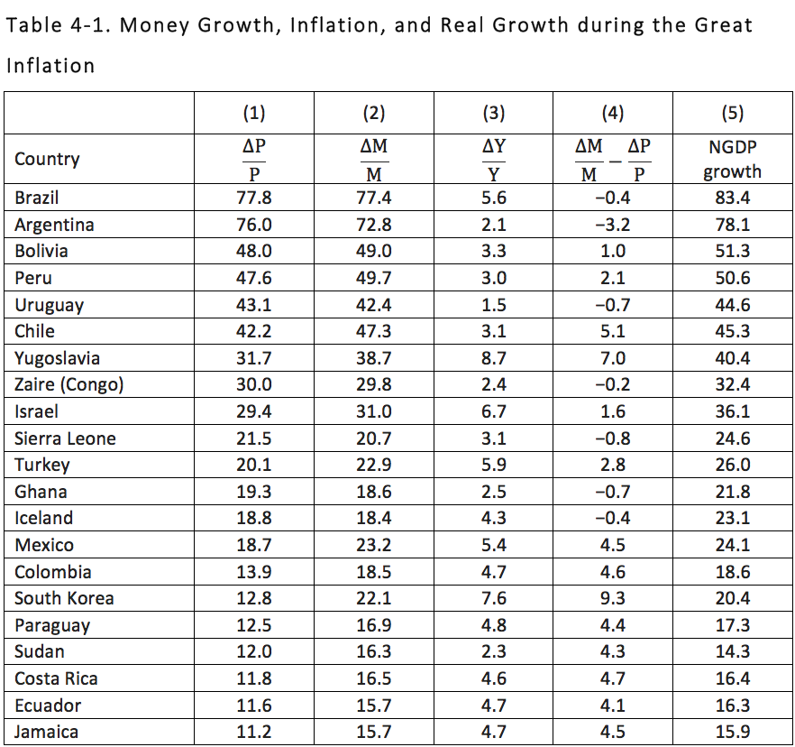
In Brazil and Argentina, prices were doubling approximately every 15 months, for decades on end.
In pre-modern times, the value of various goods tended to bounce around, rising one year and then falling the next. That’s actually still true for most goods, if you define “value” in relative terms. Thus even in countries with high inflation persisting for decades, the relative price of commodities like copper or oranges doesn’t show any dramatic (long run) upward or downward trend.
But whereas this pattern was true for essentially all goods in pre-modern times, in modern times we see two examples of goods that experienced a very rapid decline in value, which persisted over many decades. These two goods are computer chips and fiat money.
For many decades, the price of computer chips has been falling in half every 18 months, on average. This tendency is called “Moore’s Law.” In some developing countries during the 20th century, the price of their currency has been falling in half every 18 months, on average, for many decades. By 1990, one unit of Brazilian or Argentine currency could be purchased at a far lower price than in 1950, almost regardless of what you used to buy the currency. The price of their currency fell in terms of apples, oranges, coal, iron, US dollars and Japanese yen.
Over time, computer chip makers found it possible to produce a billion chips at the same cost that they had previously produced a million chips. Fiat money countries found that they could produce a trillion or even a quadrillion pesos at the same cost as they formerly produced a million or billion pesos. That cost reduction was a necessary but not sufficient cause of hyperinflation. You also needed to actually produce the money. Unlike computer firms, not all central banks are profit maximizers. (Thank God!)
It’s possible to measure NGDP using any numeraire. Thus you sometime see people claim that China has the world’s second largest GDP. In yuan terms, China’s GDP is much larger than the US GDP in dollar terms. So when people say China has the second largest GDP, they are implicitly describing what China’s GDP would look like if priced in terms of US dollars (without a PPP adjustment). Similarly, you could describe China’s GDP if priced in terms of ounces of gold or silver or one pound bags of rice. Or computer chips.
If you described the US or China’s GDP in terms of computer chips, it would be rising astronomically, it would look like a country experiencing hyperinflation. But the US and China don’t have hyperinflation. Venezuela has hyperinflation. And that’s because hyperinflation occurs when a country’s price level is rising very rapidly in terms of the thing in which prices are actually denominated.
Imagine I drew 100 graphs; each showing the US GDP measured using a different numeraire. One graph showed GDP in dollar terms. Another in terms of gold. Another in terms of apples. Another in terms of toasters. And one graph showed US GDP in terms of computer chips.
Now suppose I asked you to explain why America’s GDP in terms of computer chips rocketed much higher, year after year, for decades. Would you make reference to the Phillips Curve? To an “overheating economy”? Obviously not. Indeed I’m attacking a straw man here.
When we look at actual inflation and NGDP growth in money terms, almost nobody uses the Phillips Curve to explain inflation in a country experiencing hyperinflation. During the famous German hyperinflation of 1920-23, the world’s most famous non-monetarist economists, people like Keynes and Wicksell, suddenly switched to describing inflation in entirely monetarist terms. And then when the hyperinflation ended, Keynes quickly went back to non-monetarist explanations of inflation.
It’s always been known assumed that hyperinflation is a special case, which can only be explain by looking at what’s going on with a country’s currency. Similarly, hyperinflation of prices when measured using computer chips as a numeraire can only be explained by referring to things like Moore’s law, not Phillips curves. Hyperinflation is nothing more than a currency losing value at a very high rate. The debate is over how to explain “normal” inflation, normal NGDP growth rates.
The following equation is always and everywhere precisely true, to the very last decimal point:
M*V = C + I + G + (X-M)
Understanding what this equation means and more importantly what it doesn’t mean is the key to understanding money/macro.
The equation reminds me of two large hoofed male animals with curved horns, bashing their heads into each other, over and over again. NGDP is determined by M*V!! No it’s determined by C + I + G!!
LOL. It’s an identity!
Tags:
18. October 2020 at 21:29
“For many decades, the price of computer chips has been falling in half every 18 months, on average. This tendency is called “Moore’s Law.” ”
Moore’s Law: ‘is the observation that the number of transistors in a dense integrated circuit doubles about every two years.’
19. October 2020 at 02:37
Not that I’d say this is entirely true, just a useful aide memoire to understanding – for me at least. From, originally, Frances Coppolla.
“Hyperinflation is really the hypervelocity of money.”
Derived from knowing that the money in your hand will be worth less next week, tomorrow, heck maybe this afternoon. So spend it, right now. So it’s not entirely derived from the quantity of money…..or perhaps we might say when that M leads to substantial changes in V.
19. October 2020 at 03:43
If what Tim Worstall says is true, then we could have a super-hyper inflation in the future.
That is, today people can order everything online.
Sheesh, that being the case, you better order everything even before you get your Friday paychecks, and stock up on staples for a year ahead.
No need for wheelbarrows; your mouse can spend more money in an hour than you can in a year on foot.
Still, German 10-year bonds offer minus 0.62%. UST at the mirror-image at 0.62%, on the plus side.
For 40 years, the Temple of Orthodox Macroeconomic Theology has held sermons, or maybe seances, on pending break-outs in inflation.
Oldsters will remember Lucy and Charlie Brown, and the football….
19. October 2020 at 04:24
Scott,
love these mind-benders. And I am hyper-jealous that you’re about a decade or so older than me and still produce such incredibly original ways of looking at the world… while my ability to do the same is really going downhill lately.
19. October 2020 at 04:30
‘In pre-modern times, the value of various goods tended to bounce around, rising one year and then falling the next.’
Depending on one’s definition of ‘pre-modern times,’ I believe that a lot of this variation was due to weather affecting agriculture. Good years, good harvests, low prices; bad years, bad harvests, high prices. As well as higher disposable income for landowners in good years, etc.
19. October 2020 at 06:33
Yes it is an identity. I like to say it is an accounting equivalency. When I studied economics courses, I do not recall this being taught as such——in other words it was as if each side of the equation represented some kind of cause and effect statement.
It reminds me of a good friend of mine who has 2 masters degrees from Columbia in Physics and Math. He was a straight A student. He told me that it was not until many years later that he realized SINE was just a ratio between 2 specific sides of a triangle—opposite over hypotenuse.
He was outraged!—-Kind of funny——but he had a point. He started a Tutor school, which he has had for 30 years to make sure this would never happen to another student.
19. October 2020 at 06:59
I’d not thought of this:
“That is, today people can order everything online.
Sheesh, that being the case, you better order everything even before you get your Friday paychecks, and stock up on staples for a year ahead.
No need for wheelbarrows; your mouse can spend more money in an hour than you can in a year on foot.”
That 30 days interest free balance on a credit card becomes something that can’t really be sustained in a hyperinflationary world. Or can it? Anyone actually know what has happened to that sort of thing in highly inflationary environments?
On the other side, something from the past. Early 1990s Russia, selfemployed taxes were paid 12 months in arrears. Or perhaps 8 months after tax year end, that sort of thing. Which when inflation is 1000 and 2000 % a year is a pretty good deal for the self employed.
19. October 2020 at 07:43
Re: “M*V = C + I + G + (X-M)”
M*Vt is a subset and proxy for N-gDp. M*Vt = AD. That’s why you calculate rates-of-change to measure AD relative to N-gDp.
The calculation is simple arithmetic. The lags are math constants (not long and variable).
Money should be defined exclusively in terms of its means-of-payment attributes. The present array of interest-bearing checking accounts has confused the distinction between means-of-payment accounts (the primary money supply) and saving-investment accounts and created a dilemma as to what portion, if any, of these interest-bearing accounts should be considered as savings.
This dilemma is resolved when the transactions velocity of demand deposits is taken into account; i.e., deposit classifications are analyzed in terms of monetary flows (M*Vt). Obviously, no money supply figure standing alone is adequate as a “guide post” to monetary policy.
See: New Measures Used to Gauge Money supply WSJ 6/28/83
“The specialists recognize something called “true money” – money that is spent. And they have long kept track of various money supply categories know as M1, M2, M3, and L.
But opinions vary widely on what M1 and the other, broader Fed measures really mean. The measures are designed to resolve some of the confusion by isolating money intended for spending, the money held as savings. The distinction is important because only money that is spent-so-called “true money” – influences prices and inflation.”
Like Dr. William Barnett said (a former NSA Rocket Scientist), “the Fed should establish a “Bureau of Financial Statistics”.
19. October 2020 at 08:55
Tim, You cited this:
“Hyperinflation is really the hypervelocity of money”
This is basically wrong, as you can see from the table I included. Hyperinflation is maybe 99% money printing and 1% velocity boosting.
But yes, V does rise during hyperinflation.
mbka, Mine is going downhill too.
Tacticus, Yes.
19. October 2020 at 09:43
I rarely pay with cash but I forgot my wallet the other day and luckily I had a $20 bill in my car to buy food. In the change I received a dime from 1966 and so I quickly Googled to see if it had silver in it. Apparently they stopped putting silver in dimes in 1965 and the relevant federal act is the Coinage Act of 1965 eliminated silver from circulating coinage…and there is an economic law associated with all of this called Gresham’s law.
19. October 2020 at 10:17
Scott: Moore’s Law and the Phillips Curve should be mentioned together more often since the BLS has monetized a vital connection between them.
The deflation procedure used by the BLS to calculate the PPI entails estimating the market price change of an item and adjusting that change by monetizing changes in the that item’s quality as estimated by the BLS. This results in the real price of the item being greater or lesser than the change in the market price. It is of course the market price change before the quality change that is the basis of most economic relationships, e.g., supply=demand, inputs=outputs, income=spending, calculation of profit and loss.
The real dollar change increased by these quality changes are fantasy dollars but they have an impact because they are the basis for the deflation of NGDP. These fantasy dollars increase the real dollar value of RGDP but do not impact nominal values in any way and thus they decrease measures of inflation. The impact of this is an increase in the output and employment of items with quality increases which show in the Phillips curve the unexpected drop in unemployment along with a drop in inflation, something we have been experiencing for decades.
This deflation process also warps the relationship between wages and productivity (the latter is a result of the BLS PPI deflators).
I have not seen this mentioned as a reason for the Phillips Curve acting the way it has especially since the growth in Tech. Nor have I seen any interest on the part of economists to have the BLS quantify the impact that its deflation process has on RGDP.
19. October 2020 at 11:22
Gene, I remember that step. That a was a NECESSARY condition for the Great Inflation.
Art, You said:
“It is of course the market price change before the quality change that is the basis of most economic relationships, e.g., supply=demand, inputs=outputs, income=spending, calculation of profit and loss.”
Good point, and I’d add that this is one motivation for NGDP targeting.
And I see in the next paragraph you allude to that too.
I’m not sure, however, that this can explain the recent Phillips curve puzzles. Here’s why. If you replace inflation with NGDP growth, you avoid that bias from flawed inflation estimates. But a Phillips curve linking unemployment with NGDP growth looks almost equally puzzling in recent years.
I’m sticking with my view that the Phillips curve is simply a highly flawed model. True in some cases, but by no means a general model of the business cycle. Not a good forecasting tool.
19. October 2020 at 12:30
sumner, so I looked up Gresham’s Law and it is “bad money drives out good money”. So when we took silver out of our coins those coins stopped circulating because the “melt value” was worth more than the face value of the coin—so the post 1965 dimes (bad money) drove out the silver dimes (good money). I have spent a lot of time in the Caribbean and the Eastern Caribbean and Bahamian dollars are pegged to the US dollar. So their currency derives value from the fact it can be traded in not for silver but for an American dollar. So if I paid for something in Nassau with American dollars they would always say “sorry, we only have Bahamian money for change.” And related is what I was buying in Nassau was Johnnie Walker Black Label which if the proverbial s hits the fan could be used as currency because everyone knows the price the world over and it retains its value.
19. October 2020 at 14:31
“It is of course the market price change before the quality change that is the basis of most economic relationships, e.g., supply=demand, inputs=outputs, income=spending, calculation of profit and loss.”
No, of course.
“The focus on equilibrium and prices is due to the hypothetico-axiomatic method, a.k.a. the deductive methodology. The axioms are postulated that people are individualistic and focus on maximising their own satisfaction (named ‘utility’, in honour of Jeremy Bentham, the first economist to argue for the legalisation of the then banned practice of charging interest; Bentham, 1787). Next, a number of assumptions are made: perfect and symmetric information, complete markets, perfect competition, zero transaction costs, no time constraints, fully flexible and instantaneously adjusting prices. McCloskey (1983) has argued that economics has been using mathematical rhetoric to enhance the impression of operating scientifically. Equilibrium will not obtain, if only one of the axioms and assumptions fails to hold. But their accuracy is not tested. Yet, one can estimate the probability of obtaining equilibrium.
Despite the claims to rigour, the pervasive equilibrium argument and focus on prices reveal a weak grasp of probability mathematics: Since for partial equilibrium in any market, at least the above eight conditions have to be met, if one generously assumed each condition is more likely to hold than not – corresponding to a probability higher than 50%, for instance, 55% – then the probability of equilibrium equals the joint probability of all conditions, which is 0.55 to the power of 8: less than 1%. As the probability of each of the eight conditions being an accurate representation of reality is likely significantly lower than 55% (most having a probability approaching zero themselves), it is apparent that the probability of partial equilibrium in any one market approaches zero (Werner, 2014b). For equilibrium in all markets, these very low probabilities have to be multiplied by each other many times. So we know a priori that partial, let alone general equilibrium cannot be expected in reality. Equilibrium is a theoretical construct unlikely to be observed in practice. This demonstrates that reality is instead characterised by rationed markets. These are not determined by prices, but quantities: In disequilibrium, the short side principle applies: whichever quantity of supply and demand is smaller can be transacted, and the short side has the power to pick and choose with whom to trade (not rarely abusing this market power by extracting ‘rents’, see Werner, 2005).1
Without equilibrium, quantities become more important than prices.”
https://www.sciencedirect.com/science/article/pii/S0921800916307510#bb0295
19. October 2020 at 15:06
Interesting table. That column 1 and column 2 are similar (that is M change is similar to P change) supports what I think you said about the monetary policy regime determining prices. Each measurement in the table is probably the annual average within an inflation episode for a given country. A geometric average might be superior to an arithmetic average and it is uncertain which was presented. Some of these episodes might have lasted many years but not necessarily the entire 40 years to 1990. Depending upon the meaning of long term, it could be said this is not long term data.
I will link a graph that shows the central bank balance sheet as a percentage of GDP by bank (country). The numbers are disparate. I think M is related to the total balance sheet for each central bank. If the total balance sheet numbers are disparate then M is likely also disparate.
Does this graph in some way support the idea that in the long run prices are not determined by M?
https://imgrz.com/item/cb-balance-sheet.dN29
19. October 2020 at 15:30
Brian, That table shows that M and P are by no means perfectly correlated. That’s why it works best for hyperinflation episodes.
19. October 2020 at 16:07
I was surprised how closely correlated are column 1 and column 2 in your table. M really does matter.
When I say long term I have always meant very long term like the sun will run out of fuel soon.
19. October 2020 at 17:58
Great post, Scott!
Your identity gets to the heart of differences between MM versus NKE thinking. IMO: MM economists evaluate the economy in the context of the ***definition*** of aggregate demand (MV = Py) whereas NKE always start from a Keynesian ***theory*** of AD: y = c(r, y) + i(r, yt- q) + g …. For New Keynesian economists (most economists, even a lot who claim they are not Keynesians) NGDP is just a some residual forecast for an appendix after they run their RGDP forecast through an Okun gap and then a Phillips curve model to pop out inflation. Sadly this roundabout approach leads one to easily forget that NGDP ***is*** aggregate demand.
And consequently to forget that G can’t boost AD unless monetary conditions (ie mainly the central bank) allows it to boost M or V.
Alas these are all things I’ve learned from reading your posts and other MMs.
19. October 2020 at 20:35
Scott, I just want to straighten out one thing: Coming straight after the reference to Keynes and Wicksell changing their tunes before and after the german hyperinflation, I presume you are being ironic in writing, “It’s always been known that hyperinflation is a special case, which can only be explain by looking at what’s going on with a country’s currency.” ?
19. October 2020 at 23:44
“And consequently to forget that G can’t boost AD unless monetary conditions (ie mainly the central bank) allows it to boost M or V.”
Quite right {according to Prof. R.A.Werner}?
“ . . . whereby the coefficient for ∆g is expected to be close to –1. In other words, given the amount of credit creation produced by the banking system and the central bank, an autonomous increase in government expenditure g must result in an equal reduction in private demand. If the government issues bonds to fund fiscal expenditure, private sector investors (such as life insurance companies) that purchase the bonds must withdraw purchasing power elsewhere from the economy. The same applies (more visibly) to tax-financed government spending. With unchanged credit creation, every yen in additional government spending reduces private sector activity by one yen. “
“Equation (22) indicates that the change in government expenditure ∆g is countered by a change in private sector expenditure of equal size and opposite sign, as long as credit creation remains unaltered. In this framework, just as proposed in classical economics and by the early quantity theory literature, fiscal policy cannot affect nominal GDP growth, if it is not linked to the monetary side of the economy: an increase in credit creation is necessary (and sufficient) for nominal growth.
Notice that this conclusion is not dependent on the classical assumption of full employment. Instead of the employment constraint that was deployed by classical or monetarist economists, we observe that the economy can be held back by a lack of credit creation (see above). Fiscal policy can crowd out private demand even when there is less than full employment. Furthermore, our finding is in line with Fisher’s and Friedman’s argument that such crowding out does not occur via higher interest rates (which do not appear in our model). It is quantity crowding out due to a lack of money used for transactions (credit creation). Thus record fiscal stimulation in the Japan of the 1990s failed to trigger a significant or lasting recovery, while interest rates continued to decline. ”
http://eprints.soton.ac.uk/339271/1/Werner_IRFA_QTC_2012.pdf
20. October 2020 at 02:50
OT
Well maybe no hyperinflation…and no more hyperventilating either.
Everybody says Biden is going to win.
I will miss stories like this:
“Elsewhere on the campaign trail, President Donald Trump downplayed reports of struggles in fundraising, telling a rally that he could raise a billion dollars in a day if he had to, for example by extorting the money from Exxon Mobil (NYSE:XOM) in return for a couple of drilling licenses.”
—30—
No more TDS responses.
When one gets older, life gets duller. And now Biden as President.
Shuffleboard, anyone? How about listening to Gertrude reprise her hernia again? Did you know there is a new clerk at the 7-11?
20. October 2020 at 06:00
I don’t see the point of the comparison. It makes sense to increase the output of computing power as fast as possible given the cost of doing so. The cost of creating money so close to zero that it’s optimal rate of production has to be governed by the effect on real income.
20. October 2020 at 06:02
re: “That table shows that M and P are by no means perfectly correlated”
How close to you need to get? Why couldn’t you apply that outcome to N-gDp level targeting?
20. October 2020 at 06:09
Neutrality of money is the idea that a change in the stock of money affects only nominal variables in the economy such as prices, wages, and exchange rates, with no effect on real variables, like employment, real GDP, and real consumption. – Wikipedia
Basically, the non-neutrality of money is where R-gDp increases faster than inflation. There’s no “sweet spot” in hyperinflation.
20. October 2020 at 06:21
N-gDp targeting minimizes real output and maximizes inflation. It is obvious without calculation that real output increases before inflation exerts itself. The FOMC’s Covid-19 response is proof. Therefore it is also obvious that the monetary authority should target R-gDp, not N-gDp.
Furthermore, without a model you have no basis for debate.
20. October 2020 at 06:40
Lending via the banks using new money products is endogenous. Lending by the nonbanks via savings products is exogenous. Lending by the banks debases nominal incomes. Lending by the nonbanks expands real incomes.
Idled and bottled up savings reduces Vt. Money products cannot offset idled savings (monetary savings), because they are inherently inflationary (finance predominately existing products).
20. October 2020 at 09:14
Thanks Alex. The key is that aggregates are generally measured in money terms, not gold or computer chip terms. That’s why we care about money.
Rajat, I should have said “It’s always been assumed that hyperinflation is a special case”. In my view, it isn’t.
20. October 2020 at 09:49
re: “That’s why we care about money”.
Economists don’t care. You get mathematicians like William Barnett, of divisia monetary aggregates, trying to apply math to ill-defined terms.
There has always existed professional sanction for a variety of bias and ignorance: MSB ‘s balances in the MCBs were designated as interbank demand deposits (IBDD’s – balances maintained by customer banks in correspondent banks), presumably because MSBs were called banks and were insured by the FDIC and not the FSLIC (and not counted in M1).
At the same time Savings and Loan’s deposits were insured by the FSLIC and their balances in the MCBs were not designated as IBDDs (were counted in M1); neither institution had the right to hold deposits transferable by check on demand, without notice, and without income penalty (the legal basis for becoming a MCB), prior to the DIDMCA; both were the customers of the MCBs; and neither had REG Q ceiling restrictions prior to 1965.
Guess what’s wrong after the DIDMCA?
20. October 2020 at 09:53
When you consider the increase in money velocity, decrease in demand for money, since 2/1/2020, there should be an upward surge in stocks and the economy.
1/1/2020 ,,,,, 5.86
2/1/2020 ,,,,, 5.99
3/1/2020 ,,,,, 5.35
4/1/2020 ,,,,, 4.59
5/1/2020 ,,,,, 4.56
6/1/2020 ,,,,, 4.36
7/1/2020 ,,,,, 4.25
8/1/2020 ,,,,, 4.23
9/1/2020 ,,,,, 4.16
“Driving equity allocations higher in 2021 will in part be driven by a robust economic recovery from the COVID-19 pandemic, with GDP growth estimated to be 5.8%, according to Goldman.”
20. October 2020 at 09:59
There are 6 seasonal, endogenous, economic inflection points each year.
(they may vary a little from year to year):
Pivot ↓ #1 3rd week in Jan.
Pivot ↑ #2 mid Mar.
Pivot ↓ #3 May 5,
Pivot ↑ #4 mid Jun.
Pivot ↓ #5 July 21,
Pivot ↑ #6 2-3 week in Oct.
These seasonal factors are pre-determined by the FRB-NY’s “trading desk” operations, executing the FOMC’s monetary policy directives: in the present case just reserve “smoothing” and “draining” operations, the oscillating inflows and outflows, the making and or receiving of correspondent and other interbank payments by and large using their “net free” (as opposed to “net borrowed”) excess reserve balances).
Onward and upward.
21. October 2020 at 09:51
Scott: Thanx for responding to my comment. You are certainly more articulate than I am. I totally agree with your reliance on nominal dollars and that was the attempted point of my comment. I don’t understand how economists can use BLS deflated data. Monetizing quality changes in deriving PPI deflators corrupts every aspect that “real” dollars touch.
The BLS creates fantasy dollars that have no connection with the market. It is not only the Phillips Curve but every variable, relationship, model that use real dollars that have been derived with PPI deflators are tainted. The fantasy dollars derived by PPI deflators increase the measures of real output and decrease the measures of inflation.
Why don’t economists at least have the BLS publish the the extent fantasy dollars impact in total and each industry so the extent of its influence can be seen?
21. October 2020 at 10:19
Art, Thanks. In my view the fundamental problem here is that we don’t know what we are trying to measure when we estimate inflation, and tech is a good example. What does it even mean to say the quality adjusted prices of TVs is down 98%? since 1960? Quality measured how?
In principle, we’d want to measure how much more income you’d need each year to maintain steady utility, but we don’t have clue as to how to measure utility. People actually enjoyed those 1960s TV sets! For that reason, all “quality adjustments” become highly subjective.
All this was less of a problem in 1980 when inflation was double digits. If measured inflation was 13% but actual inflation was 11% or 15%, it was still high. But if measured inflation is 2% and actual inflation is 0% or 4%, that’s a big difference in relative terms.
21. October 2020 at 13:46
So quite obviously, the prices of computer chips have not actually been falling for a long time. Instead, manufacturers have been producing chips that have long exceeded what the market actually needs (4-core, 8-core chips for smartphones). The price of memory chips has inexplicably even been rising at times. So the analogy is severely flawed.
Moore’s law departed from having an impact on chip prices more than a decade ago.
21. October 2020 at 19:02
Michael, I don’t think you understand Moore’s Law. It’s not the price of a single chip, it’s the price of a given amount of computer power that’s falling. I used the term ‘chip’ loosely. I think most readers understood what I meant.