One of the ways that macro differs from micro is that macro is essentially a branch of history.  Micro is not.  And yet today’s macroeconomists often have not studied monetary history.  Marcus Nunes and Ramesh Ponnuru directed me to a paper by White House economics advisor Jason Furman:

A decade ago, the prevalent view about fiscal policy among academic economists could be summarized in four admittedly stylized principles:

1. Discretionary fiscal policy is dominated by monetary policy as a stabilization tool because of lags in the application, impact, and removal of discretionary fiscal stimulus.

2. Even if policymakers get the timing right, discretionary fiscal stimulus would be somewhere between completely ineffective (the Ricardian view) or somewhat ineffective with bad side effects (higher interest rates and crowding-out of private investment).

3. Moreover, fiscal stabilization needs to be undertaken with trepidation, if at all, because the biggest fiscal policy priority should be the long-run fiscal balance.

4. Policymakers foolish enough to ignore (1) through (3) should at least make sure that any fiscal stimulus is very short-run, including pulling demand forward, to support the economy before monetary policy stimulus fully kicks in while minimizing harmful side effects and long-run fiscal harm.

Today, the tide of expert opinion is shifting the other way from this “Old View,” to almost the opposite view on all four points.

I think this is right, but where Furman and I differ is on the desirability of this shift.

Furman refers to the view “a decade ago” but he might just as well have said 90 years ago.  The New Keynesian consensus is actually not all that far from the views of progressive economists back in the 1920s, which favored a price level target and were skeptical about fiscal policy.  After the 1930s, opinions moved in the old Keynesian direction.  It wasn’t until the 1960s that the tide started swinging away from the “vulgar Keynesian” view that fiscal policy was more important than monetary policy.  Friedman and Schwartz started he counterrevolution, and by the 1990s it was pretty much complete.  Stabilization policy should rely on monetary policy.

And now we have still another swing of the pendulum, back toward the old Keynesian views of the post-1936 period. Here’s Furman:

The New View of fiscal policy largely reverses the four principles of the Old View—and adds a bonus one. In stylized form, the five principles of this view are:

1. Fiscal policy is often beneficial for effective countercyclical policy as a complement to monetary policy.

2. Discretionary fiscal stimulus can be very effective and in some circumstances can even crowd in private investment. To the degree that it leads to higher interest rates, that may be a plus, not a minus.

3. Fiscal space is larger than generally appreciated because stimulus may pay for itself or may have a lower cost than headline estimates would suggest; countries have more space today than in the past; and stimulus can be combined with longer-term consolidation. 

4. More sustained stimulus, especially if it is in the form of effectively targeted investments that expand aggregate supply, may be desirable in many contexts.

5. There may be larger benefits to undertaking coordinated fiscal action across countries.

Those old Keynesian views of the late 1930s were rejected for lots of good reasons.

I’m not quite sure what is more humiliating for the profession of macroeconomics:

1.  That we keep making the same mistakes, over and over again.

2.  That we change our views of macro on “new information”, which in fact is not new to anyone with an even passing interest in macro history.  (I.e., who know that the temporary QE of 1932 had little impact, just as the more recent temporary QE had little effect.)

3.  That we don’t pay attention to the empirical studies that refute old Keynesianism.

4.  That many macroeconomists are not even aware of the cyclical nature of their field.

It’s not unusual to find this sort of cyclicality in the arts.  For instance, in the arts there are swings back and forth between a more “classic” style and a more “romantic” style.  But it’s kind of embarrassing to see this in a science.

(And don’t embarrass yourself by arguing macroeconomics is not a science.  Of course it’s a science.  It’s failed science, but then so are some of the other sciences, at least based on what I’ve read about the crisis in replication.  The term ‘science’ is not a compliment, it’s not some sort of award given to a field, like a Nobel Prize.  It’s simply a descriptive term for a field that builds models that try to explain how the world works.  Saying that science must be successful to be viewed as science is as silly as saying that a work of art must be good to be considered art.)

We need a “timeless” macro.  That is, theories should not be developed to meet the specific conditions in the economy, at that moment.  And yet that’s exactly what old Keynesianism is, which is why it goes in and out of style.  Instead, theories should be developed to explain the entire history of macroeconomics—the full data set.  If your model is not good at explaining hyperinflation, stagflation, liquidity traps and the Great Moderation, then it’s not a good theory.

Old Keynesianism is not a good theory.

PS. I’d like to congratulate Ben Klutsey for winning the Great Communicators Tournament in Washington DC on Wednesday night. Some of you may know that David Beckworth and I both participate in the Mercatus Center’s Program on Monetary Policy. Unfortunately we both live some distance from the headquarters in Arlington, VA. Ben is the program’s manager, and does a lot of the behind the scenes work that readers might not be aware of. I feel lucky to work with someone who is both a very nice guy and a highly talented manager.

Also congratulations to runner-up Charles Blatz, another Mercatus employee.

Over at Econlog I did a post discussing the austerity of 1946.  The Federal deficit swung from over 20% of GDP during fiscal 1945 (mid-1944 to mid-1945) to an outright surplus in fiscal 1947.  Policy doesn’t get much more austere than that! Even worse, the austerity was a reduction in government output, which Keynesians view as the most potent part of the fiscal mix.  I pointed out that employment did fine, with the unemployment rate fluctuating between 3% and 5% during 1946, 1947 and 1948, even as Keynesian economists had predicted a rise in unemployment to 25% or even 35%—i.e. worse than the low point of the Great Depression.  That’s a pretty big miss in your forecast, and made me wonder about the validity of the model they used.

One commenter pointed out that RGDP fell by over 12% between 1945 and 1946, and that lots of women left the labor force after WWII.  So does a shrinking labor force explain the disconnect between unemployment and GDP?  As far as I can tell it does not, which surprised even me.  But the data is patchy, so please offer suggestions as to how I could do better.

Let’s start with hours worked per week, the data that is most supportive of the Keynesian view:

Weekly hours worked dropped about 5% between 1945 and 1946. Does that help explain the huge drop in GDP?  Not as much as you’d think. Here’s the civilian labor force:

So the labor force grew by close to 9%, indicating that the labor force in terms of numbers of worker hours probably grew.  Indeed if you add in the 3% jump in the unemployment rate, it appears as if the total number of hours worked was little changed between 1945 and 1946 (9% – 5% – 3%).  Which is really weird given that RGDP fell by 22% from the 1945Q1 peak to the 1947Q1 trough–a decline closer to the 36% decline during the Great Contraction, than the 3% fall during the Great Recession.

That’s all accounting, which is interesting, but it doesn’t really tell us what caused the employment miracle.  I’d like to point to NGDP, which did grow very rapidly between 1946 and 1948, but even that doesn’t quite help, as it fell by about 10% between early 1945 and early 1946.

Here’s why I think that the NGDP (musical chairs) model did not work this time. Let’s go back to the hours worked, and think about why they were roughly unchanged.  You had two big factors pushing hard, but in opposite directions. Hours worked were pushed up by 10 million soldiers suddenly entering the workforce.  In the offsetting direction were three factors.  A smaller number of (mostly women) workers leaving the workforce, unemployment rising from 1% to 4%, and average weekly hours falling by about 5%.  All that netted out to roughly zero change in hours worked.

So why did RGDP fall so sharply?  Keep in mind that while those soldiers were fighting WWII, their pay was a part of GDP. They helped make the “G” part of GDP rise to extraordinary levels in the early 1940s.  But when the war ended, that military pay stopped.  Many then got jobs in the civilian economy.  Now they were counted as part of hours worked. (Soldiers aren’t counted as workers.)  That artificially depressed productivity.

It’s also worth noting that real hourly wages fell by nearly 10% between February 1945 and November 1946:

This data only applies to manufacturing workers. But keep in mind that the 1940s was the peak period of unionism, so I’d guess service workers did even worse.  So my theory is that the sudden drop in NGDP in 1946 was an artifact of the end of massive military spending, and the strong growth in NGDP during 1946-48, which reflected high inflation, helped to stabilize the labor market.  When the inflation ended in 1949, real wages rose and we had a brief recession.  By 1950, the economy was recovering, even before the Korean War broke out in late June.

Obviously 1946 was an unusual year, and it’s hard to draw any policy lessons.  At Econlog, I pointed out that the high inflation occurred without any “concrete steppes” by the Fed; T-bill yields stayed at 0.38% during 1945-47 and the monetary base was pretty flat.  Some of the inflation represented the removal of price controls, but I suspect some of it was purely (demand-side) monetary—a rise in velocity as fears of a post-war recession faded.

This era shows that you can have a lot of “reallocation” and a lot of austerity, without necessarily seeing a big rise in unemployment.  And if you are going to make excuses for the Keynesian model, you also have to recognize that most Keynesians got it spectacularly wrong at the time.  Keynesians often make of big deal of Milton Friedman’s false prediction that inflation would rise sharply after 1982, but tend to ignore another monetarist (William Barnett, pp. 22-23) who correctly forecast that it would not rise.  OK, then the same standards should apply to the flawed Keynesian predictions of 1946.

Tyler Cowen used to argue that 2009 showed that we weren’t as rich as we thought we were.  I think 1946 and 2013 (another failed Keynesian prediction) show that we aren’t as smart as we thought we were.

Update:  David Henderson has some more observations on this period.

I’ve finally had a chance to read Paul Romer’s critique of macroeconomics, and it’s every bit as interesting as you might expect.  I’m going to focus on a single issue, which in my view lies at the heart of what’s gone wrong in recent decades—identification.  This issue has been the main focus of my blogging over the past 7 1/2 years, so it’s very dear to my heart. By late 2008, it was clear to me that not only did economists not know how to identify monetary shocks, but also that they were very far off course, and didn’t even understand that fact. Indeed this misunderstanding actually became highly destructive to progress in both economic science and economic policymaking.  One of the two the worst contractionary monetary shocks of my lifetime is generally regarded as “easy money”.  So how did we get here?

1. The earliest monetary shocks were seen as involving the price of money.  Coin debasement was a common example.  No one knew the money supply, and banks did not yet exist. This policy tool was used by FDR in 1933, but today has fallen out of fashion in big economies. Small countries like Singapore still use the price of money (exchange rates) as a policy instrument, but they do not drive the research agenda.  I’m trying to bring it back with NGDP futures targeting.

2.  Although the monetarist approach to identification (i.e. the money supply) dates back at least to Hume, it really came into its own with fiat money, especially during hyperinflationary fiat regimes.  Milton Friedman preferred the M2 money supply as a monetary indicator, at least during part of his career.

3.  Then for some strange reason the profession shifted from the money supply to interest rates, as an indicator of monetary shocks.  But why?

Perhaps you are thinking that you know the answer.  Maybe it had something to do with the early 1980s, when velocity was unstable and monetarism was “discredited”.  If that is indeed what you are thinking, then it merely illustrates that you are even more confused than you know.  Yes, velocity is unstable.  And yes, that means Friedman’s 4% money growth rule might not be a good idea.  But that has absolutely no bearing on the argument for replacing the money supply with interest rates, as an indicator of the stance of monetary policy.

The relationship between i and NGDP is just as unstable as the relationship between M2 and NGDP, probably more unstable.  At least with M2, we generally can assume that an increase means an easier monetary policy, and a reduction means a tighter policy.  We don’t even know that much about the relationship between interest rates and NGDP. Right now, markets expect about a 1% fed funds rate in 2019. Suppose you had a crystal ball that told you that the fed funds rate in 2019 would be 3%, not 1%.  There’s a classic “monetary shock”. The stance of monetary policy changed unexpectedly.  But which way—is that easier than expected policy, or tighter?  I have no idea, and you don’t know either.  Even worse, my best guess would be “easier” but the official model says “tighter.”

Paul Romer says we know that monetary shocks are really important.  I agree.  And he says the Volcker disinflation proves that.  I agree, and could cite many other examples, probably even more than Romer could cite.  So I’m completely on board with his general critique of those who claim we don’t know whether monetary shocks are important.  But Romer then claims that the real interest rate is a useful measure of the stance of monetary policy, and it isn’t—not even close.

Am I denying that if the Fed suddenly raised the real interest rate by 200 basis points, money would be tighter on that particular day or week?  No, I agree that that statement is true.  But it’s also true that if the Fed suddenly raised the nominal interest rate by 200 basis points, money would be tighter on that particular day or week.  Or if the Fed suddenly cut M2 by 10%, money would be tighter on that particular day or week.

So why don’t we use M2 to measure the stance of monetary policy?  Because over longer periods of time, movements in M2 do not reliably signal easier or tighter monetary policy.  But that’s also true of movements in nominal interest rates. If you have a highly contractionary policy, then inflation and nominal rates will fall in the long run.  Hence low rates don’t mean easy money.  And this argument also applies to real interest rates.  If the Fed adopts a tight money policy that drives the economy into a depression, then real interest rates will decline, even as policy is effectively contractionary.  This actually happened in 1929-33 and 2008-09.

All of the traditional indicators are unreliable.  The smarter New Keynesians will say that money is tight when the interest rate is above its Wicksellian equilibrium rate. But how do we know when that is the case?  After all, the Wicksellian equilibrium rate cannot be directly observed.  You need to look at outcomes; Wicksell said interest rates were above equilibrium when prices were falling, and vice versa. But that means we can only identify easy and tight money by looking at outcomes; are prices rising or falling?

Today we would substitute above or below 2% inflation, or 4% NGDP growth, but the basic idea is the same.  Money is tight when it’s too tight to hit your target, and vice versa. Ben Bernanke got this right in 2003, and then lost track of this concept when he joined the Fed:

Do contemporary monetary policymakers provide the nominal stability recommended by Friedman? The answer to this question is not entirely straightforward. As I discussed earlier, for reasons of financial innovation and institutional change, the rate of money growth does not seem to be an adequate measure of the stance of monetary policy, and hence a stable monetary background for the economy cannot necessarily be identified with stable money growth. Nor are there other instruments of monetary policy whose behavior can be used unambiguously to judge this issue, as I have already noted. In particular, the fact that the Federal Reserve and other central banks actively manipulate their instrument interest rates is not necessarily inconsistent with their providing a stable monetary background, as that manipulation might be necessary to offset shocks that would otherwise endanger nominal stability.

Ultimately, it appears, one can check to see if an economy has a stable monetary background only by looking at macroeconomic indicators such as nominal GDP growth and inflation. On this criterion it appears that modern central bankers have taken Milton Friedman’s advice to heart.

Others will object that New Keynesians understand that it’s the level of interest rates relative to the Wicksellian equilibrium rate that matters.  For instance, a recent paper by Vasco Curdia shows that money was actually quite contractionary, during and after the Great Recession.

Yes, but that paper was written in 2015.  Back in late 2008 and throughout 2009, market monetarists were just about the only people claiming that monetary policy was highly contractionary—and that was the period when we most needed clear thinking.  Others were lulled by meaningless indicators like low nominal and real interest rates, as well as a ballooning monetary base.

How did we end up using interest rates as an indicator of the stance of monetary policy?  Romer provides one possible clue in his paper:

By rejecting any reliance on central authority, the members of a research field can coordinate their independent efforts only by maintaining an unwavering commitment to the pursuit of truth, established imperfectly, via the rough consensus that emerges from many independent assessments of publicly disclosed facts and logic; assessments that are made by people who honor clearly stated disagreement, who accept their own fallibility, and relish the chance to subvert any claim of authority, not to mention any claim of infallibility.

I fear that economists have deferred too much to the “central authority” of central banks.  When I talk to macroeconomists, they seem to think it’s natural to use interest rates in their monetary models because the central banks actually target short-term interest rates.  But that’s a lousy reason.

Another problem may be that some economists are infected by a popular prejudice—that low interest rates are a “good thing” for the economy.  We visualize that we would be more likely to buy a new house if interest rates fell, and extrapolate from that to the claim that low rates would boost GDP.  That’s obviously an example of the fallacy of composition.  Yes, I’d be more inclined to borrow money if interest rates fell, ceteris paribus.  But some other guy is less inclined to lend me the money if interest rates fell, ceteris paribus.  Of course ceteris is not paribus if interest rates fall, and it all depends on whether they fall because of an increase in the money supply (expansionary) or more bearish expectations from the public (contractionary.)

Elsewhere I call this “reasoning from a price change”, and even Nobel laureates do it:

Real interest rates have turned negative in many countries, as inflation remains quiescent and economies overseas struggle.

Yet, these negative rates haven’t done much to inspire investment, and Nobel laureate economist Robert Shiller is perplexed as to why.

“If I can borrow at a negative interest rate, I ought to be able to do something with that,” he tells U.K. magazine MoneyWeek. “The government should be borrowing, it would seem, heavily and investing in anything that yields a positive return.”

But, “that isn’t happening anywhere,” Shiller notes. “No country has that. . . . Even the corporate sector, you might think, would be investing at a very high pitch. They’re not, so something is amiss.”

And what is that?

“I don’t have a complete story of why it is. It’s a puzzle of our time,” he maintains.

Actually there is no puzzle.  Shiller seems unaware that it’s normal for the economy to be weak during periods of low interest rates, and strong during periods of high interest rates.  He seems to assume the opposite.  In fact, interest rates are usually low precisely during those periods when the investment schedule has shifted to the left.  Shiller’s mistake would be like someone being puzzled that oil consumption was low during 2009 “despite” low oil prices.

I know what commenters will say—I’m a pigmy throwing stones at Great Men. They are right.  Guilty as charged.  Look, I’ve made the mistake of reasoning from a price change numerous times—it’s easy to do.  But that won’t stop me from criticizing the ideas of people much more famous than I am.  In Paul Romer I’ve found a kindred spirit.

PS.  Since I’m nearly 6’4″, perhaps I should be PC and add, “Not that there’s anything wrong with being a pigmy”.

PPS.  This link has videos to the recent Mercatus/Cato conference on monetary policy rules.

James Bullard has a new paper out discussing the NeoFisherian perspective on interest rates.  According to the NeoFisherian view, holding interest rates at a low level for a long period of time will lead to persistently low inflation rates. That’s because (according to the Fisher effect) nominal interest rates tend to be correlated with inflation rates, at least in the long run.

James Bullard says he used to hold the opposite view:

Indeed, during the past six years I have warned, along with many others, that the Committee’s ZIRP has put the U.S. economy at considerable risk of future inflation. In fact, my monetarist background urges me to continue to make this warning right now!

Actually, Milton Friedman would have been dismissive of that view:

Low interest rates are generally a sign that money has been tight, as in Japan; high interest rates, that money has been easy.

Instead, the view that Bullard attributes to monetarists is actually the Keynesian/Austrian view.  It’s Keynesians and Austrians who reason from a price change.  They are the ones who insist that low interest rates are expansionary.

The NeoFisherians had a perfect opportunity to fix this flaw in macroeconomics, but instead fell into the trap of making exactly the opposite mistake.  NeoFisherism is also an exercise in reasoning from a price change, but in their case they assume that low rates are disinflationary, not inflationary.  That is, they assume that low rates are tight money, whereas Keynesians and Austrians tend to assume it’s easy money.  It’s neither.

If the NeoFisherians are going to make any headway convincing outsiders, then need to do two things that Bullard failed to do in his paper:

1.  Discuss the Keynesian/Austrian/Monetarist view of the liquidity effect.  Why have central bankers assumed for decades, even for hundreds of years, that lower rates are expansionary?  Are they really that delusional?  There are literally 100s of natural experiments where central banks adjusted interest rates unexpectedly.  In each case we can observe the market reactions. How do exchange rates react? How do commodity prices react? How do TIPS spreads react? The Bullard paper, and other papers I’ve seen on NeoFisherism, simply glosses over these key questions. But these are exactly the questions that skeptics would want answered.

2.  NeoFisherians need to provide a plausible example of a shift toward lower rates leading to a lower inflation environment.  The example provided by Bullard is not at all persuasive, for reasons outlined by Ryan Avent:

Where I think Mr Bullard begins to go off course is in treating the Fed’s behaviour like a zero-interest-rate peg. Yes, interest rates have been below 0.5% for nearly eight years, and the Fed has consistently promised to raise rates gradually. But it has promised to raise rates gradually, which is not the sort of thing a zero-rate targeting central bank would do. More importantly, markets have believed that the Fed would raise rates. When the fed fund futures contract for July 2016 began trading back in 2013, markets reckoned that the interest rate set at the July meeting would be in the neighbourhood of 1.5% to 2%. That was in line with the dots published by the Fed at the time. The Fed told markets that rates were going up, and markets saw no reason to disbelieve.

As it turned out, both markets and the Fed were far too optimistic; over time the expected path of rate hikes has been both pushed forward into the future and it has flattened. Markets now think that the fed fund rate will be no higher than 1% three years hence. Maybe this shift has occurred because the Fed has signalled more strongly that it is pursuing a zero-rate peg, but I doubt it; in every published projection since 2013, the dots have continued to rise up to some “normal” rate well above zero.

I would argue that Mr Bullard is wrong; it is not the case that the Fed is choosing low rates and inflation expectations are therefore converging toward a low level. I would argue that the Fed has been targeting very low inflation, and falling inflation expectations imply much lower interest rates in future.

This dynamic is there back in 2013. In its projections the Fed indicates that rates will rise steadily, even as it projects that inflation will be extraordinarily low, just over 1% in 2013, converging, finally, toward 2% by the end of 2015. Essentially every set of Fed projections since then has shown the same thing. It allowed its QE programmes to end despite too-low inflation, and it raise its interest rate in December despite too-low inflation. The Fed has signalled very strongly that markets should expect inflation to remain at very low levels, indeed, below target. It would be shocking if inflation expectations hadn’t trended inevitably downward.

Now return to the Fisher equation. If the global real interest rate is in the neighbourhood of 0% and expected inflation is in the neighbourhood of 1%, that suggests the Fed will have an extremely difficult time raising nominal interest rates beyond 1%. Mr Bullard has the regime right, but the causation wrong. The Fed has driven the economy into this rut in its determination to keep inflation low.

I agree with Ryan Avent, except that last part about the difficulty the Fed would have in raising inflation.

In fact, there is a good example of NeoFisherian in action, which occurred just last year.  As we will see, it is consistent with my previously expressed interpretation of NeoFisherism, and not consistent with the views of either NeoFisherians, or anti-NeoFisherians.  The truth is orthogonal to the debate.  Both sides are missing the point.  Whether low rates are expansionary or contractionary depends entirely on whether they are achieved via an expansionary or a contractionary monetary policy.

It recently occurred to me that Switzerland circa January 2015 is an almost perfect example of NeoFisherianism is action.   In previous posts I argued that the perfect NeoFisherian policy had two parts:

1.  A promise to gradually appreciate the currency against a major currency, which would reduce interest rates via the Interest Parity Theorem.

2.  A simultaneous once and for all large appreciation in the currency, which would exert a contractionary impact on prices that was large enough to prevent an immediate rise in the price level from the lower interest rates caused by step #1.

So step #1 reduces long run inflation via the PPP effect, and step #2 prevents Dornbusch-style overshooting in the short run.  The Swiss didn’t announce precisely this policy, but the policy they did announce was virtually identical in all meaningful respects—and it had exactly the effect predicted by the NeoFisherians (but not for the reasons they assume).  Here’s what Switzerland did to interest rates in January 2015:

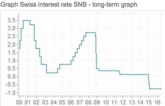
Notice that interest rates fell from 1/8% to negative 3/4%, almost immediately. Because of interest parity, that created an expectation that the Swiss franc would gradually appreciate over time, which leads investors to expect lower trend inflation in Switzerland, compared to neighboring countries.

But how did the Swiss authorities make sure this decrease in interest rates had a contractionary impact?  The answer is simple; they did a simultaneous, once and for all, massive appreciation in the SF.  Not a formal appreciation through government fiat, but rather by switching from artificial peg of 1.2 SF to the euro, to a floating exchange rate.  The market (correctly) took this as a signal of tighter money, and the SF promptly rose by about 10% to 15% against the euro.  But they could have achieved the same effect by simply revaluing the SF upward by the same amount, by fiat.

The upshot of all this activity was a sharp decline in Swiss inflation:

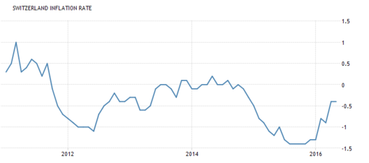
A skeptic might argue that inflation fell for some other reason, say falling oil prices. That might be part of it, but on the very day the new policy was announced, I recall people predicting slower RGDP growth and lower inflation, and they were correct.  I’m confident that if a Swiss CPI futures market had existed, then CPI futures would have declined on this policy change.

So the Swiss got exactly the result predicted by the NeoFisherians.  A Keynesian skeptic will say; “Yes, both interest rates and inflation fell, but the lower interest rates did not actually cause the lower inflation.  Indeed ceteris paribus the lower interest rates raised inflation, but the sharp appreciation of the SF put even more downward pressure on inflation.”

The problem with this argument is that whenever market interest rates decline, things are never ceteris paribus.  Let’s take the standard Keynesian interpretation of an open market purchase.  Say the Fed unexpectedly increases the monetary base by 2%, and this causes nominal interest rates to decline.  Is the policy inflationary?  Probably yes, but not for the reason that Keynesians assume.  Other things equal, the lower interest rates will tend to lower velocity, and hence will tend to lower inflation.  More than 100% of the heavy lifting for higher NGDP comes from the 2% increase in the base, and less than 0% comes from the lower interest rates.

The preceding point isn’t even controversial; it’s part of the standard monetary economics 101 literature.  But macro has moved so far in an interest rate oriented direction that many people have forgotten these basic truths, or else they never even learned them.  Blame Woodford if you wish.  I blame almost the entire profession.  In any case, yes, it’s actually the appreciation of the SF, not the lower interest rates, which causes lower inflation.  But it’s also true that it’s the increase in the money supply, not the lower interest rates, that cause higher inflation in the standard Keynesian policy case.

Some will complain that my example only works in the special case of exchange rate manipulation, and that NeoFisherism does not work in a closed economy.  Not so. Instead of a sudden appreciation of the SF, the Swiss could have achieved the same contractionary result by combining lower interest rates with:

1.  Lower official gold prices (A reverse of FDR’s 1933 technique).

2.  A promise to increase the money supply at a slower rate, from now until the end of time.

3.  A lower price of NGDP futures contracts (which would first have to be created.)

4.  Appointing a crazy hawk like Bob Murphy to be head of the SNB.

Basically, you need to combine a lower interest rate with something else that creates the expectation of tighter money going forward.

It’s not a question of whether the Keynesians or the NeoFisherians are right—I don’t agree with either group.  It’s a question of which types of monetary policy shocks produce which results.  I see three interesting cases:

1.  The Keynesian case:  In this case, an easy money policy causes a reduction in both short and long-term interest rates.  Inflation tends to rise.

2.  The NeoFisherian case:  In this case, a tight money policy causes a fall in short and long-term interest rates.  Inflation tends to fall.

3.  The Monetarist case:  In this case, an easy money policy causes short-term rates to fall and long-term rates to rise.  Inflation tends to rise.

As soon as you are able to visualize the monetarist case as being a hybrid Keynesian/NeoFisherian case, you know you are on the right track. If you see the monetarist case as being short run Keynesian and long run NeoFisherian, then you “get it.” If not, reread the post.

PS.  I’ve already indicated that January 2015 in Switzerland was a NeoFisherian case.  I’d add that the January 2001, September 2007 and December 2007 Fed FOMC policy announcements were all Monetarist cases.  Short and long rates moved in opposite directions. There are also lots of Keynesian examples, but I can’t recall one at the moment.

PPS.  I’ve simplified things by assuming that central banks normal lower rates by open market purchases, that is, an increase in the base.  They can also reduce market interest rates by lowering the tax on bank reserves, i.e. by lowering IOR. Nothing important changes in this case, but it’s even harder to see the irrelevancy of interest rates when monetary policy shifts from base supply control to base demand control.

PPPS.  I may turn this post into a paper, so I’d appreciate any serious feedback.

For years, I’ve been trying to convince the profession that inflation is not the right variable, it’s NGDP growth that matters. One example I frequently cite is the prediction of NK models that inflation caused by negative supply shocks can be expansionary at the zero lower bound.  The failure of the NIRA during the 1930s suggests that this is not true, and now a new NBER study by Julio Garin, Robert Lester and Eric Sims reaches the same conclusion:

The basic New Keynesian model predicts that positive supply shocks are less expansionary at the zero lower bound (ZLB) compared to periods of active monetary policy. We test this prediction empirically using Fernald’s (2014) utilization-adjusted total factor productivity series, which we take as a measure of exogenous productivity. In contrast to the predictions of the model, positive productivity shocks are estimated to be more expansionary at the ZLB compared to normal times. However, in line with the predictions of the basic model, positive productivity shocks have a stronger negative effect on inflation at the ZLB.

The basic problem here is that expected inflation doesn’t matter, what matters is expected NGDP growth.  And while a positive supply shock does indeed reduce inflation, that sort of disinflation is the good kind.  What really matters is NGDP growth, which is not reduced by positive supply shocks.

Here’s one implication they draw from their study:

In the meantime, since our empirical results are difficult to square with the textbook theory, caution seems to be in order when advocating for policies such as forward guidance and fiscal stimulus, both of which are predicted to be highly expansionary when policy is constrained by the ZLB.

BTW, if economists seriously want to argue that inflation matters, they really ought to come up with a coherent definition of inflation.  So far they have failed to do so.