What monetary recessions don’t look like

This post is a sort of response to a Tyler Cowen post entitled “Japan slides into recession,” even though I don’t actually disagree with his comments:

“Japan’s economy contracted at a much-worse-than-expected 3.7% annualized rate in the January-March period, tipping the country into a recession as the March 11 earthquake and tsunami caused declines in consumer spending, business investment and private-sector inventories.”

The article is here.  . . . The simple lesson is that earthquakes and tsunamis are contractionary, not expansionary.  This is a classic example of real business cycle theory and how it can also apply to economies which are, in some regards, still in Keynesian corridors.

It is certainly true that natural disasters don’t help an economy, by creating jobs rebuilding the damage.  But it’s also true that recessions caused by real shocks like natural disasters look nothing like recessions caused by tight money.  For one thing, they don’t necessarily reduce future expected NGDP, and hence the economy tends to recover quickly.  The big drop in 1st quarter GDP was largely due to an unprecedented plunge in March industrial production–down 15.3%.  When you consider the fact that the tsunami occurred on the 11th, it seems likely that IP fell over 20% in the last two thirds of March.

But since then it has risen sharply, rising 1.6% in April, and 5.7% in May—the biggest jump since 1953.  Yes, it is still about 8% below February levels, but the point is that output only fell for one month.  With a monetary recession, output usually falls for 6 to 18 months.

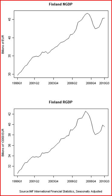
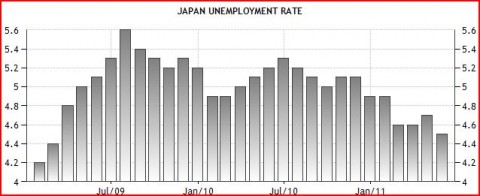
An even bigger difference shows up in the unemployment data.  Because companies know that output will quickly recover, they tend to hold on to workers.  Thus the unemployment rate has continued to fall during the “recession,” which is obviously quite unlike a monetary recession.

Why do the best arguments against the RBC model involve exchange rates?

The “real business cycle” model has led some conservatives to claim that monetary stimulus will merely lead to more inflation, not more real economic growth.  They don’t believe that nominal shocks have real effects.

The two most famous arguments against the RBC model both involve exchange rates.  One argument was discussed in a recent post by Paul Krugman.  He presented a graph showing that real exchange rates became vastly more volatile after the Bretton Woods exchange rate regime was abandoned around 1971.  You might ask: So what?  Is it any surprise that exchange rates became more volatile after the world abandoned fixed exchange rates?  It’s not surprising that nominal rates got more volatile, but real rate volatility is a bit more of a surprise.  Recall that the RBC model predicts that nominal shocks won’t have real effects.  (Indeed even some non-RBC types like Milton Friedman didn’t expect such dramatic volatility.)

A second example was recently discussed by Ryan Avent; the famous study (by Barry Eichengreen) that showed countries tended to begin recovering from the Great Depression precisely when they left the gold standard.  Again, if nominal shocks don’t have real effects (as some RBC proponents claim), then this pattern is hard to explain.

I don’t recall anyone explaining why economists use foreign exchange data to refute the extreme RBC view that nominal shocks don’t matter.  After all, nominal shocks are also supposed to have real effects in closed economies.  Why not use a more conventional indicator of monetary stimulus, such as the money supply, or interest rates, or the inflation rate?  One answer is that it’s very hard to identify monetary shocks using those indicators.  Low rates may reflect easy money, or they may reflect a weak economy expected as a result of tight money.  A big increase in the money supply might reflect easy money, or might be the Fed accommodating more demand for base money in response to past deflationary policies.  The rate of inflation might rise due to supply shocks, or due to demand shocks.

In the interwar period there was a pretty good correlation between money, prices, and output, as there were big monetary shocks that led to procyclical movements in the price level.  That looks good for conventional demand-side models.  But postwar data is less clear.  Now the monetary authority tries to offset changes in velocity, so money and prices are much less clearly correlated with output.

Exchange rates are almost ideal in two respects.  Unlike interest rates and the money supply, a rising value of the dollar is a relatively unambiguous indicator of tighter money, and vice versa.  And unlike changes in inflation, it’s pretty easy to separate out changes in exchange rates that reflect exogenous policy decisions, and those that reflect other factors.  For instance, both the abandonment of the gold standard, and the abandonment of Bretton Woods were pretty clearly exogenous policy decisions.  Indeed they were “monetary policy” broadly defined to include “changes in the international value of one’s money.”

I prefer NGDP, but many of my critics say that indicator assumes away the question.  How do we know central banks can influence NGDP? I think that’s wrong, especially if you use expectations, but nevertheless exchange rates are clearly something that governments can control.

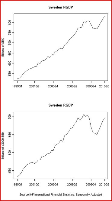
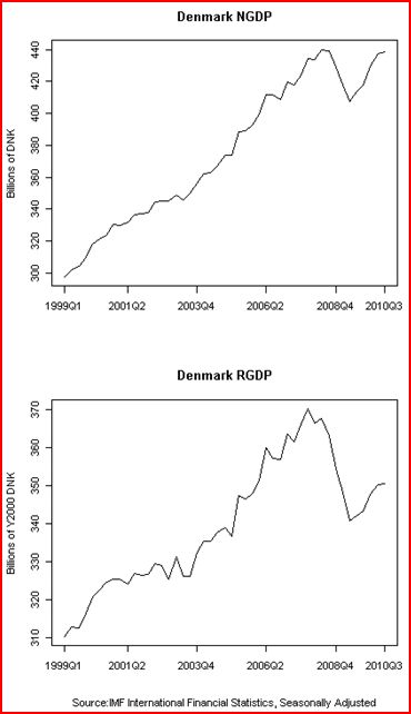
I recently mentioned some very suggestive data for Sweden and Denmark, and a commenter named Justin Irving (a student at Uppsala University) sent me data which repeats the two famous experiments that I cited above, albeit in a slightly less impressive way (only three observations.)  He sent me graphs showing NGDP and RGDP for three major Nordic countries.  (Norway was not included, presumably because its vast oil wealth would make it an unrepresentative country.)
.

.

.

.

.

.

.

.

.

.

.

.

.

.

.

.

.

.

.

.

.

.

.

.

.

.

.

.

.

.

.

.

.

.

.

.

.

.

.

.

.

.

.

.

.

.

.

.

.

.

.

.

.

.

.

.

.

.

.

.

.

.

In 2008 both Denmark and Finland were either in the euro, or fixed to the euro.  Sweden was floating, and as soon as the recession hit it allowed the krona to depreciate sharply.  As you can see from the graphs above, Sweden’s NGDP grew significantly faster than the other two.  This is no surprise; both RBC and conventional macro models would predict this result.  But now look at RGDP growth.  The RBC model suggests that devaluing a currency will simply result in higher inflation, not faster RGDP growth.  Yet it’s clear that Sweden did much better than Denmark and Finland in terms of RGDP.  Why is that?  I believe the faster NGDP growth caused the faster RGDP growth.  A real business cycle proponent would presumably say it was just coincidence, just as it was coincidence that America started recovering in 1933 and France began recovering in 1936, etc.  Lots of interesting coincidences.

All these natural tests of the RBC model lead me to wonder what we can infer from the fact that economists use exchange rates, not conventional monetary indicators, when attempting to refute the RBC.  What does that tell us about contemporary monetary economics?  Here are some answers:

1.  Postwar conventional macro models that identify monetary shocks on the basis of interest rates or money supply changes are not reliable.  Instead when researchers want convincing evidence they reach back to the definition of monetary policy provided by that “monetary crank” of the 1930s, George Warren.  Warren proposed that monetary shocks were changes in the price of gold.

2.  We need a variable that gives a clear and unambiguous indication of changes in the stance of monetary policy (like exchange rates), and which also can be measured in real time, (like exchange rates.)

3.  The best way to get that variable would be for the Fed to create and subsidize a NGDP (and RGDP) futures market.

No longer would we have to wait for serendipitous experiments like the staggered ending of the gold standard, or the end of Bretton Woods.  We’d have a perfect real time indicator of monetary shocks.  We could observe how Fed actions (and policy speeches) impacted NGDP futures prices.  We could observe how changes in NGDP futures impacted various real variables.  The actual parameters of all sorts of macro models would lay naked and exposed, like the skeleton of a dead animal lying in the midday Libyan sun.  Want to know the slope of the SRAS?  Is Plosser right or is Krugman right?  Just compare the reaction of RGDP and NGDP futures to a sudden Fed announcement that under the pressure of regional Fed presidents, QE2 was being ended prematurely.  Something tells me that Plosser would not be happy with the answer that the markets would give him.

The experiments discussed by Krugman and Avent tell us something important (and unpleasant) about modern RBC models.

The fact that those experiments had to rely on exchange rate shocks tells us something important (and unpleasant) about modern conventional macro.

More evidence the recession was not caused by the financial crisis

Last night I criticized a new Robert Hall article in the JEP, which argued that the financial crises of 1929 and late 2008 caused the Great Depression and the Great Recession.  I pointed out that there was no financial crisis in 1929, and that it was the Depression that caused the later banking panics.  I pointed out that the 2008 recession was well advanced before the banking crisis of late 2008 occurred.  Undoubtedly those crises worsened each slump by further depressing AD, but they weren’t the cause—tight money was.

Soon after I read a new article by Lee Ohanian from the same journal that supported my argument regarding the Great Depression, and provided lots of new evidence for the current recession.  Here he points out that the Great Depression could not have been caused by the financial crisis:

For example, many cite the fact that the number of U.S. banks declined by about 40 percent between 1929 and 1933 as a central reason why the Great Depression was “Great,” and draw inferences from this fact for the potential effect of financial crises more generically (for example, Reinhart and Rogoff, 2009). But most of the Depression-era banks that closed were either very small or merged, which indicates that the decline in banking capacity resulting from bank closings during the Depression was small. In fact, the share of deposits in banks that either closed or temporarily suspended operations for the four years from years 1930-1933 was 1.7 percent, 4.3 percent, 2 percent, and 11 percent, respectively (Cole and Ohanian, 2001).

Moreover, the Depression was indeed “Great” before any of the monetary contraction or banking crises identified by Friedman and Schwartz (1963) occurred.  Figure 2 shows that industrial hours worked had declined by 29 percent between January 1929 and October 1930, which is not only before the first Friedman and Schwartz-identified banking crisis (November 1930 to January 1931), but is also before the money stock fell.

I agree with Friedman and Schwartz that the 1930s banking crises were important, but only because they led to the hoarding of base money, not for Bernankean disintermediation reasons.  Indeed Ohanian misses his strongest argument here—the 1933 crisis was worse than all the others put together, yet 1933 was the first year of recovery, seeing brisk growth in industrial production and prices.  You might argue; “But that’s because dollar devaluation pushed up AD in 1933.”  Bingo—it’s all about AD, not disintermediation.  Then Ohanian turns his attention to the current crisis:

The corporate sector typically has nearly as much cash as they invest in plant and equipment, and cash is relatively high during the last few years.

One possible issue with Figure 3, however, is that perhaps the cash reserves displayed in the figure are only being held in certain sectors while other sectors have little or no cash. To address this issue, Chari and Kehoe (2009, in progress) examine firm-level data from Compustat to compare firms that use external finance to those that do not. These data indicate that on average about 84 percent of investment is financed internally. Indeed, about two-thirds of investment is undertaken by firms not using external funds, and slightly more than half of the investment undertaken by those using external funds is still financed internally.  .  .  .

Another assertion often made in the financial explanation is that small firms have much less access to capital markets, and thus small firms decline much more than large firms during crises. However, Cravino and Llosa (2010, in progress) show that there is virtually no change at all in the relative sales performance of small versus large firms during the 2007-2009 recession. They compare the share of sales accounted for by small, medium, and large firms during the fourth quarters of 2007, 2008, and 2009. The shares are virtually identical in these periods, indicating that firm sales growth was unrelated to firm size. This fact is thus inconsistent with a central assumption in the financial explanation.

The financial explanation also argues that the 2007-2009 recession became much worse because of a significant contraction of intermediation services. But some measures of intermediation have not declined substantially. .  .  .  bank credit relative to nominal GDP rose at the end of 2008 to an all-time high. And while this declined by the first quarter of 2010, bank credit was still at a higher level at this point than any time before 2008.6 Similarly, flow of funds data show that borrowing levels of households and of the nonfinancial businesses that households own, are virtually unchanged since 2007, and that the composition of those liabilities across mortgages and other liabilities are also unchanged. These data suggest that aggregate quantities of intermediation volumes have not declined markedly.  But perhaps the most challenging issue regarding the financial explanation is why economic weakness continued for so long after the worst of the financial crisis passed, which was around November 2008

I’ve consistently argued that if the AD was there then firms would have supplied the output, and I think most business people would tell you the same thing.  Many have pointed to a Rogoff-Reinhart study that shows financial crises are usually followed by severe recessions.  I have responded by asking “how many of those financial crises were associated with a sharp currency appreciation?”   I believe the answer is “damn few,” and I often cite the US in the early 1930s, Argentina in 1998-2002, and the US in the last half of 2008.  Note that in all three cases the financial crisis was caused by tight money, and in the first two cases rapid growth resumed almost immediately after the currency was devalued.  Here’s how Ohanian addresses the evidence:

From the perspective of the financial explanation, the continuation of recession long after the worst of the crisis passed raises an important puzzle about why employment did not recover sooner. This question is not resolved simply by noting that economies often remain below trend for years following a significant financial crisis (Cerra and Saxena, 2008; Blanchard, 2009). In many of these cases, output remains below trend because productivity is far below trend (Ho, McGrattan, and Ohanian, 2010, in progress). But as documented above, the productivity deviation during the 2007-2009 U.S. recession was very small, which means that low productivity is not the reason why U.S. macroeconomic weakness continued.

Ohanian explores whether the Great Recession can be explained in a “neoclassical” (i.e. real business cycle) framework.  He argues that the data on hours worked, productivity, etc, indicate that the marginal rate of substitution between labor and leisure had fallen far below the marginal productivity of labor.  He speculates that various government policies might have created an implicit tax wedge in the labor market that discouraged employment.  In my view this explanation suffers from some of the same problems as the financial disintermediation story—it doesn’t explain the sharp fall in NGDP and RGDP after June 2008.  But in making his argument he keeps scoring points that indirectly support my alternative wage/price stickiness story.  It’s like some alternative universe version of TheMoneyIllusion.  We both agree that the standard story is wrong.  We both agree on why it is wrong.  But we disagree on which alternative story is better.  I believe Ohanian has a very persuasive critique of the disintermediation story, and I very much want Ohanian to win in his attempt to discredit the mainstream story.  Then the dispute will be between my sticky wage/price transmission mechanism for falling AD, and his tax wedge argument that relies on the sort of explanation put forth by people like Casey Mulligan:

A policy explanation for the 2007-2009 recession is that economic policies, including the 2008 tax rebate, the Troubled Asset Relief Program (TARP), the American Recovery and Reinvestment Act (ARRA), Cash for Clunkers, Treasury mortgage modififi cation programs, and other policies signififi cantly contributed to the recession. The common argument here is that these policies distorted incentives through their deficient design and also increased uncertainty about the underlying economic environment. . . .

For example, Mulligan (2010a) studies the possible effect of U.S. Treasury mortgage modification programs on the low employment rate by evaluating how the eligibility requirements for these programs implicitly raised income tax rates on some households to levels of more than 100 percent.

I think I know which alternative explanation will win out among mainstream economists.   🙂

PS.  I did find one flaw in the Ohanian article.  He seems to assume that US productivity did much better than German productivity during the recession.  But this may be because he was only able to find employment data for Germany (which did not decline) whereas hours worked data in Germany (which did decline) might have told a different story